KPI 用於 Analog Circuit Design

Analog circuit desing is not an art (or only partly is an art).

Majority day-to-day life is normal.  How come it is so difficult????

Because there is a big gap between device level and final result!!!

這是一個認知的間題

 

3 layers of knowledge in analog circuit

 

1. Device level

gm, rout, Cc

ft = gm/Cc;   gain = gm * rout

 

 

 

3. Result and 現象

Oscillator: oscillate or not and lock time, frequency detune

PLL: lock or not and lock time, spur, phase noise

ADC: ENOB, SNDR

 

Problem ==>

1. Need lot of simulation time: garbage in; garbage out!!

2. No physical insight!!!!

Because a big gap between device parameter and result/現象

 

Solution ==> Bridge the gap using KPI

What is KPI?

between device parameters and final results

only a few (2-4 parameters)

A clear coorelation between KPI and final results (best if there is a math formula)

CentOS 常用軟體

Use VMware to install CentOS 4.8 on windows 7

 

Step 1: Install vmware-toolbox on linux, not sure what this toolbox is useful??

network --> bridged mode, very slow?  How about hostonly and NAT?  What's the tradeoff?

Now using bridged mode and works OK.

Step 1.1: Make sure sshd service is on.  And install putty in PC so that can remote control.

 

Step 1a: If need to install the latest update, do “yum update”.  However, this may not be necessary

Step 1b: Some rpm package is NOT in the default repo (check /etc/yum.repo.d).  Need to install other rpm repo.

Some popular rpm repo:   rpmforge (e.g. mercurial),  Ruby.repo (Ruby jam)

==> rpmforge:  http://wiki.centos.org/AdditionalResources/Repositories/RPMForge

A.   Get http://packages.sw.be/rpmforge-release/rpmforge-release-0.5.2-2.el5.rf.i386.rpm

B.   rpm --import http://apt.sw.be/RPM-GPG-KEY.dag.txt   (get the GPG key)

C.   rpm -K rpmforge-release-0.5.2-2.el5.rf.*.rpm  (verify the package A)

D.  rpm -i rpmforge-release-0.5.2-2.el5.rf.*.rpm  --> check /etc/yum.repo.d/rpmforge.repo exist

 

Step 2: Install VNC server on linux, very useful tool.  However, need to change default twm to gnome-session.  Install ultravnc or realvnc on PC.

Very useful tool:  Host: need to change /etc/sysconfig/vncservers;  Make sure vncserver serivce is running, and editing .vnc/xstartup file.

Can use netstat -lt to check the tcp port status.

It's very useful that pc copy and paste can use directly on linux.   Just run "vncconfig" in linux and make sure all options are checked and keep the vncconfig ON ALL TIME then it works!!

(make sure the correct setting on unltravnc and realvnc are checked, too)

 

2a: Editing /etc/sysconfig/vncservers file to support multiple users, window size, and resolutions:

### /etc/sysconfig/vncservers #################

VNCSERVERS="1:root 2:alu 3:atd"
VNCSERVERARGS[1]="-geometry 800x600"
VNCSERVERARGS[2]="-geometry 1024x768 -depth 24"
VNCSERVERARGS[3]="-geometry 800x600"

###########################################

 

2b: Use putty login as root, alu, atdl; setting password for each users (very important!! Otherwise service won’t start).

2c:  Start the vnc service as root ==> service vncserver restart

2d: Check system->Administration->Security Level and Firewall->other ports –> add 5901,5902,5903

2d: use putty login, editing /home/alu/.vnc/xstartup as follows:

##################################################

centos4:~/.vnc> more xstartup

#!/bin/sh

# Uncomment the following two lines for normal desktop:
unset SESSION_MANAGER
exec /etc/X11/xinit/xinitrc

#[ -x /etc/vnc/xstartup ] && exec /etc/vnc/xstartup
#[ -r $HOME/.Xresources ] && xrdb $HOME/.Xresources
#xsetroot -solid grey
#vncconfig -iconic &
#xterm -geometry 80x24+10+10 -ls -title "$VNCDESKTOP Desktop" &
#twm &

##################################################

 

One annoying thing is hostname doesn't seem to work.  Need to use IP address for putty and vnc.  However, the IP address is dynamically changed because it's from DHCP server.  How to set hostname instead of using IP address? 

I did the following but not working.  How PC can know the hostname?

First, set the hostname, e.g. : centos5  system->administration->network->DNS->Hostname->centos5

This is corresponding to /etc/sysconfig/network: HOSTNAME

Then, system->administration->network->Devices->Edit->Hostname (optinal): –>centos5

This is corresponding to /etc/sysconfig/network-script/ifcfg-eth0: DHCP_HOSTNAME –> centos5

Then, system->administration->network->Devices->Edit->DNS:192.168.1.1

This is corresponding to /etc/resolv.conf

 

Step 3: Install Samba server on centos.  Samba server is not default on in centos.  Need to use yum install samba first. 

Please refer to vbird's suggestion for configuration.  Samba is based on NetBIOS, not tcp/ip.  It seems to avoid the hostname problem.

step 3(a):  yum install samba   --> rpm –qa  to check samba (samba-common, samba, samba-client)

step 3(b): edit /etc/samba/smb.conf

step 3(c): create smbpasswd:  touch smbpasswd

step 3(d): smbpasswd –a alu  (to add password to smbpasswd)

step 3(e): disable SELinux (important!!!)

step 3(f): /etc/rc.d/init.d/smb restart (start the samba server)

 

Step 4: start license server related service in /etc/rc.local

工具有關軟體

git: Check git during centos installation?  If not pre-installed:

$ rpm -Uvh http://mirror.webtatic.com/yum/centos/5/latest.rpm

$ yum install --enablerepo=webtatic git-all

kompare: Check KDE environment during centos installation.  Or install kompare inside of latest kde rpm.  Do

$ rpm -ivh ... kde ..

kdiff3: same as kompare, but more powerful.  Get the rpm directly from web.

xls2csv: convert Excel file into csv file.  There are two versions.  One is from catdoc; the other from CPAN (perl).   The one from CPAN is better in my opinion.

Ruby:  Check ruby during centos installation. rubygems: gnuplot, fastercsv

Python: Check python during centos installation.  However, the default python of centos or redhat is not the updated version (1.7.x).  For scientific computing or other applications, it is highly recommended to use EPD (Enthought) version instead.  The EPD version is installed in a separate directory, not replacing the default version.  Remember to set the path in .tcshrc or .bashrc to invoke the EPD version.

Perl: Check Perl during centos installation.

 

CAD 有關軟體

* ns3:  http://www.nsnam.org/wiki/index.php/Installation

 

* Composer: make sure to set /etc/sysconfig/vncservers ==> xwindows setting is 24-bits or pseudo 8-bit

* Sanwork: make sure to "yum install openmotif" to avoid the error of not finding libXm.so.3

 

* Vppsim (from MIT MIke Perrott)

do yum install gcc-c++ to install g++

 

To run license of Calibre, Adit,

1. start with host mode

2. Do /tools/ixl_cal_2007.4_21.19/change-hostid.sh  (in bsh, not tcsh) to change mac id

3. Do tcsh to change to tcsh

4. Do source CALIBRE.cshrc

5. Do clic_start to start mentor related license

 

 

Step 5: Script 和 Web 有關軟體

* Ruby: centos comes with default ruby.  However, it is helpful to install rubygems, gnuplot, and other gems.

Please refer to web how to install them.  yun install ruby ruby-gems (?) ruby-devel ..

* RoR (Ruby on Rail): same as above

* Apache2 and CGI.

yum install httpd ruby ruby-devel

* then need to use make install to install mod_ruby to enable the CGI working.  (same for Python and Perl).

* Use amrita for html output generation.  It's easy for viewing purpose

 

Step 6: Support ntfs file system (終於考定, another trouble maker is lib.so…)

CentOS doesn’t support NTFS file system natively, nor extFAT (Microsoft proprietary).   It is troublesome to read external hard drive (mostly NTFS).  Even though most USB drives are still using FAT that centos supports.  However, there is a 2G(?4G) limitation on FAT file size.  It makes things difficult to do external backup in step 7.

Therefore, it is important to make centos to support NTFS file system.  It is particularly troublesome for CentOS4.  Be careful on the following steps.  Reference: http://wiki.centos.org/TipsAndTricks/NTFS

It needs to include the fuse kernel module into kernel.  因此會需要 fuse, fuse-ntfs-3g, dkms, dkms-fuse.  CentOS5.4 and newer has included fuse kernel module.  Therefore, no need for dkms and dkms-fuse.

If you do:    yum install fuse fuse-ntfs-3g dkms dkms-fuse

It will not find anything because these rpm files are not centos default repo.  These rpm files are in rpmforge. 

(1) First, download rpmforge rpm-release from:

i386: http://packages.sw.be/rpmforge-release/rpmforge-release-0.3.6-1.el5.rf.i386.rpm
x86_64: http://packages.sw.be/rpmforge-release/rpmforge-release-0.3.6-1.el5.rf.x86_64.rpm

(2) After that, run:   rpm –ivh rpmforge-release-xxx

(3)  yum install fuse fuse-ntfs-3g dkms dkms-fuse

(4) check if the running version matches with kernel

uname –r to check the current running kernel

rpm –qa | grep kernel\* | sort to check the kernel and kernel-devel

It may require to do: yum update kernel to make it match.   Make sure to reboot the machine.  Debug: https://www.centos.org/modules/newbb/viewtopic.php?topic_id=26488

(5) do /sbin/modprobe fuse   if there is no error message, it is ok.

(6) From chome VM page, check USB mass storage.  On PC, the external hard drive disappears.

(7) Do   mount –t ntfs-3g /dev/sda1 /export/usb   to mount external drive

(8) Do fdisk –l to check the parition

(9) Do umount /deve/sda1 to un-mount the external hard drive

 

Step 7: setup external backup

Follow bird’s suggestion:

PC 部份常用軟體

本文整理我的 PC 內常用軟體及設定

I. Internet 及網路和雲端軟體

1. Firefox 和 add-on: xmark, IE tab, Wikidiction

2. UltraVNC 取代 Microsoft remote desktop (家用 XP, Windows 7 不支援 remote desktop)。不過 UltraVNC 似乎容易掛掉，網路上有人建議用 WinVNC 或 RealVNC。VNC 的好處是可以用在 linux。

3. Syncplicity 及 Dropbox

4. Evernote 和 Microsoft OneNote

 

G. Google 軟體及 service

1. Google desktop

 

V. 防毒軟體

1. Avira Antivir (小紅傘)

 

T. 工具類軟體

1. Total commander: 支援 unicode，非常好用。Linux 上只有 Konqueror 可用。

2. Free commander: 類似 total commander, 免費且容易使用。不支援 unicode, 會有日文及簡體亂碼。

3. Foxit: PDF reader，比 Adobe 小且快速

4. 7zip: 免費且強大壓縮軟體

 

M. 多媒體

1. Picasa: 最棒的相片 database 軟體

2. GOM player: 最佳的 video player 軟體。取代 Microsoft Media Player, KMplayer.  類似軟體尚有 VLC，MPlayer, 和 KMplayer。說明和下載。

3. iTune: CD ripper 以及 audio database

4. Imgburner: 類似 Nero, 免費且快速，用於燒 DVD 光碟和擷取 DVD -> ISO 軟體。

5. DVDFab HD Decrypter: 擷取 DVD -> ISO 軟體, 同時破除保護。

6. DVD Shrink: 類似 DVDFab HD Decrypter。

7. Daemon Tools: 虛擬光碟機軟體，用於 player ISO 檔案。

 

P. P2P 軟體

1. uTorrent: 小且常用

 

L. Linux 軟體

1. cygwin (1.7.x): gnu+windows+cygnus 簡單的說就是在 windows 上架構 linux，對於習慣在 linux 上工作的人非常方便。

幾點需要注意：change default installation to include: openssh (in Network option), tcsh (in Shell option), xwindows (in X option).

2. VMware/Virtualbox: 除了 cygwin 以外，另外的選擇是 VMware 或 Virtulbox，虛擬的機器。VMware 是商用軟體。Virtualbox 是免費軟體。

免費 RF 軟體及阻抗匹配 (Impedance Matching)

常用的 RF Simulation 軟體如 ADS, Microwave Office, 或是 SpectreRF 動則數十萬。對於大多數 RF 工程師日常的工作實在是大材(財)小用。

本文想要介紹兩個好用而且免費的 RF simulation 軟體，以及如何用這兩個軟體來做阻抗匹配。

第一個軟體是 Smith，是由 Bern 大學的 Fritz Dellsperger 教授所提供。正式版收費 $100 元；demo 版免費，但只能用五個元件而且不能存檔。說實在話這個軟體並不值得花錢買，也只能做一些簡單的事。五個元件也差不多夠用，因此只要用 demod 版就可以了。我先用 Smith 來介紹 Smith Chart 以及幾個阻抗匹配的做法。

Smith Chart 基本介紹

可參考另一篇文章 "Smith Chart"。重點摘要如下：

1.  Open load 位於 (+1, 0), Short load 位於 (-1, 0), 50Ohm load 位於 (0, 0).

2. 上半平面為 inductive load; 下半平面為 capacitive load; x-axis 為 resistive load.  因此大多 DC open 電路的 S11 位於第四象限 (如 dipole antenna)； DC short 電路的 S11 位於第二象限。

3. VSWR = constant 在 smith chart 上是圓心在 (0, 0) 的圓。 Q=constant 在 smith chart 上是橄欖形，兩端點位於 (-1, 0) 和 (+1, 0)。

 

Smith 軟體介紹

Smith 軟體最大的缺點是只能觀察一個頻點，不過這也讓設計變得簡單而且容易了解。

Step 1: 輸入 ZL (load impedance)

開啟 smith 之後，先鍵入 ZL。有兩種方法輸入 ZL: 如果知道 ZL, 可以直接輸入 ZL 的實部 (resistive load) 和虛部 (reactive load)，如圖一；實際的情形大多是 network analyzer 量測出的 S11 參數，也可以選 reflection coefficient 配合 polar 座標輸入，如圖二。  不論是用 ZL 或 reflection coefficient, 都必須提供工作頻率。

圖一： 直接輸入 ZL (load impedance) 的實部和虛部: 實部是 84.8 Ohm (resistive load), 虛部是 -125.1 Ohm (capacitive load)。

 

 

圖二： 輸入 S11 參數的 magnitude 和 angle。Magnitude 是 0.706, Angle 部份是 -31.6 度。ZL 值圖一相同。

 

Step 2: L-match with HPF 和 LPF

最簡單的 match 就是 L-match。一般而言 L-match 可以有四種方式如圖三。分別是相交在 R=50 或 G=0.02 circles。除此之外，可以相交在 capacitive 半平面或是 inductive 半平面，一共有四種組合。

圖三：L match 的四種組合。

 

實際的情況則多半是在 R>50 (或 G>0.02) 的圓內，如 dipole antenna 和 loop anenna。此時只會有兩種 L-match 。如圖四和圖五所示，RL = 84.8 - 125.1 j, 只能先並聯電感或電容和 R=50 圓相交。再串聯電容或電感完成 input matching.  仔細觀察這兩種 L-match, 圖四是 HPF，因為串聯電容及並聯電感。圖五則是 LPF，因為串聯電感及並聯電容。至於應該用那一種 L-match，由系統決定。例如，如果要濾掉 FM 干擾，應該用 HPF L-match；反之，如果要濾掉 GSM 干擾，則應該用 LPF L-match。

圖四：L-match 使用 HPF。

 

圖五：L-match 使用 LPF。

 

L-match 理論和應用都簡單，除了達到阻抗匹配之外，還附送了一個 HPF 或 LPF。對於窄頻系統效果相當不錯。

所謂窄頻系統就是頻寬小於載波的 10%。例如藍芽, WiFi 等使用 2.4 GHz ISM band，系統頻寬遠小於 240MHz。相反的，電視所使用的 UHF (或 VHF)，頻寬從 470MHz 到 850MHz，遠遠超過載波的10%，因此是寬頻系統。

L-match 的主要缺點是只針對一個頻點做 matching。雖然對於窄頻系統效果不錯，但對寬頻系統遠端頻點的 matching/LPF/HPF 可能就不夠理想。同時在做 L-match 時，系統的 Q 值可能會變大 (寬頻會差異大，group delay 變化會增加，最好 Q=0)，對某一些系統不適合。另外有時系統需要 BPF 來濾掉所有的干擾。一個解決之道就是用 Pi 或 T-match。

 

Step 3: Pi-match 和 T-match with BPF

首先把虛部去掉 --> 84.8 - 125.1j ==> 84.8 Ohm。這可以降低 Q 值同時離 50Ohm 更近一步。因為 Zl 是 capacitive loading，一開始只能使用 serial L，限制為 T match 且加上一個 LPF。

接下來再使用 L-match，把 84.8 Ohm map 到 50 Ohm。有 LPF 和 HPF 兩種選擇。

上圖是 T-match 的 LPF (LPF + L-match LPF)。下圖則是 T-match 的 BPF (LPF + L-match HPF)。

 

究竟用 T-match (或 pi-match) 有什麼好處？主要是能將 matching 和 filter 的 Q 值分開。可以達成更寬頻的 impedance matching。

什麼時候會用 T-match 或 pi-match？當 impedance 實部大於 50-Ohm，原則上使用 T-match。當 admittance 實部大於 20mS，原則上使用 pi-match。 如上圖的黃和藍兩圈之內的部份。之外的部份，似乎用 L-match 就可以，不用做 T-match 或 pi-match。

當然可以做更複雜的變化，如 cascade 幾個 T 或 pi 或混合 T 和 Pi match，最主要的目的是達到多點的 impedance matching，比處不討論。

Smith 的 L-match 和 T-match 都是以單點為基礎，雖然簡單，但很難契合實做的需要。 RFSim99 剛好補足這一點。更重要的是，RFSim99 是一個完全免費的軟體。

 

RFSim99 軟體介紹

Step 1: 輸入 ZL (load impedance)

RFSim99 的 GUI 使用起來相當容易。可以選擇用 1-port 或 2-port 元件來輸入 load impedance。我們載入一個內建的 2-port 例子且設定頻率從 400MHz 到 800MHz (UHF band)。剛好非常類似一個 dipole antenna 如下圖。600MHz 的阻抗為 84.8-125.1j Ohm ，和前面 Smith 的例子一致。

 

Step 2: L-match with HPF 和 LPF

RFSim99 已經把 L-match 自動加在軟體中。只要選 Auto Match，同時勾選 port-1 match 和 LPF (HPF) ，就可以自動產生正確的 L-match 電路。

上圖是用 HPF 的結果，可以看到 L 和 C 值和圖四一致。S11 可以看到 600MHz 有一個很深的 notch。同時 S21 也呈現 HPF 的形狀。下圖是 Smith chart 的結果。除了在 600MHz 附近 match 不錯，大部份的頻率都不好，所以這是窄頻的 match。 L-match 的 LPF 也有一樣的問題。

 

Step 3: Pi-match 和 T-match with BPF

接下來是 T-match。不過 RFSim99 沒有 T-match 或 pi-match 的自動 matching 功能。因此，我們必須用圖六或圖七所得到的結果。先看 LPF 的 T-match。

結果好很多，從 440MHz 到 800MHz S11 基本上都在 -10dB 以下。看 Smith chart 更明顯。

 

 

接下來是 BPF 的 T-match。結果更好，低頻甚至可以到 -20dB 以下。同時 Smith chart 也十分不錯。

 

 

 

附記

Ludwig 的 "RF Circuit Design" 其中有一章專門討論 impedance matching，是我看過 RF 書中最詳細的。

可以把 impedance matching 化簡問題為 R != 50Ohm to 50Ohm matching。是否有其他 optimal matching (e.g. constant Q, etc.)

Kalman Filter and PLL

考慮如 Figure 1 個 burst mode 的 packet (任何 shared media 的傳送方式)。在 packet 最前頭都會有 1010.. 的 preamble 做為 bit/symbol synchronization。緊接在後的是事先定義好的 frame sync word 用來做為確認 lock 到對的 packet 以及 word boundary。最後才是實際的 data。這個應用 focus 在 preamble 部份 (1010..) synchronization，也就是找出 (estimate) preamble 的相位和頻率，同步之後的 data。  我們可以把問題重新定義如下：A [2pft + q]  如何根據接收端的 phase 找出發射端 f (or b = 1/(2pf) or T=1/f) and q ?

[Driessen94] 和 [Christiansen94] 兩人獨立証明了這個問題的最佳解是 Kalman filter，和二階的 PLL (PI filter)有一樣的結構。但是 Kalman filter time variant 特性比 一般 PLL 更快完成 acquistion。[Patapoutian99] 將兩人的 work 作了一個很好的整理。

Figure 1: Packet Frame Structure.

Bit Synchronization State Space Model

Figure 2 描述了這個 state-space model: 我們可以定義兩個 state variables 分別為 phase disturbance 和 frequency disturbance.  Output variable, y(k), 是 phase disturbance 加上 observation timing jitter.  同時, state-space model 中還包含了 phase 和 frequency noise.    

Figure 2: State-Space Model of Bit Synchronization.

 

Kalman Filter of State Space Model

一旦我們建立了 state space model，我們可以根據 y(k) 來估計 b(k) 和 q(k) (Kalman filter), 其解如下：

Figure 3: Kalman Filter Solution of Figure 2.

 

光從上面的方程式大概很難看出什麼名堂。K(k) 是所謂的 Kalman Gain, P(k) 是 X(k) 的 covariance matrix。重點是上述的 recursive 方程式和 2nd order PLL 有者一樣的架構 [Drissen94]。

 

Kalman Filter and PLL

Figure 4 是上述 Kalman filter 的等價 block diagram。The model includes a PI time-invariant controller followed by an integrator (remember Alper's work?  PI controller plus a slow VCXO - it's a integrator).  The Kalman filter is shown has the same structure as the 2nd order PLL.

[a(k), b(k)]' 即對應 Kalman gain, K(k).

Figure 4: Block diagram of the Kalman filter and a proportional integral PLL.

 

Bit Synchronization PLL 操作分為兩種模式：Acquisition 和 Tracking

在 Acquistion 模式，Phase 和 frequency disturbance 遠大於 process noise，Q 可以忽略不計。Kalman filter 表現如 dynamic loop bandwidth 的 PLL。開始時 loop bandwidth 會增加 ( a(k)/b(k) 變大) 以加快 acquistion 的時間。一旦鎖住 loop bandwidth 會減小 ( a(k)/b(k) 變小) 以減小最終的 phase jitter。下圖顯示這樣的一個例子： P(0|-1) 時同時有 phase 和 frequency disturbance，特別是 phase disturbance 很大 (1/12)。

 

在 Tracking 模式，Kalman Gain 會收歛到最終值。因此和 2nd order PLL 是完全等價。藉者 Kalman Gain 的幫助，可以找出最佳的 PLL 設計。

 

Follow Up Task

==> 如何將 continous PLL 和 Kalman filter 連結超來？如何設計最佳 PLL考慮 VCO noise, PFD noise, 和 sigma-delta modulator noise？如何考慮 stability？

==> How about if VCO noise is time variant?  Kalman filter should be better than PLL?

==> If adding the data after the integrator (sigma-delta or just random data), then what's the equation?? can use Kalman filter to explain it?

Analog Simulation Flow

PRESIM

schematic: composer

netlister: composer - cdl (si) : netlist

testbench: tb_dut (PVT)

simulator: hspice

processs model: t350nm, u180nm, u130nm, u110nm, u110nmAL  --> put in /home/atd/tech/...

 

tb_dut.lis  = tb_dut.sp  + netlist.spi

tb_dut.sp does not include process component (nmos, pmos), but need to include PVT, need to include process ==> change tb all the time

> make tb_dut.lis ==> update tb_dut.lis

 

netlist.spi = netlist + convt_model_process ==>  netlist only change in design phase; model_process only change occasionally

 

netlist: hard to make dependency because it's from composer.  ==> make netlist directly

> make netlist    ==> update netlist

> make tb_dut.lis  ==> update netlist.spi ==> update tb_dut.lis

 

POSTSIM

netlister: calibre

testbench: tb_dut (PVT), same as presim

simulator: hspice or Adit

processs model: t350nm, u180nm, u130nm, u110nm, u110nmAL  --> same as presim

 

tb_dut.post.lis = tb_dut.sp + netlist.post.spi

> make tb_dut.post.lis ==> update tb_dut.post.lis

 

netlist.post.spi = netlist.cal + convt_model_process

> make netlist.cal  ==> update netlist.cal

> make tb_dut.post.lis ==> update tb_dut.post.lis

Kalman Filter 簡介

Kalman 濾波器的部份，我發現網路上有一些不錯的介紹 (無法找到原作者 )，應用一引用其一。

在學習 Kalman 濾波器之前，首先看看為什麼叫「Kalman」。跟其他著名的理論（例如傅立葉變換，泰勒級數等等）一樣，Kalman也是一個人的名字，不同的是，他是個二十世紀的人。

Kalman 全名 Rudolf Emil Kalman，匈牙利數學家，1930年出生於匈牙利首都布達佩斯。1953，1954年於麻省理工學院分別獲得電機工程學士及碩士學位。1957年於哥倫比亞大學獲得博士學位。我們現在要學習的Kalman濾波器，正是源於他的博士論文和1960年發表的論文《A New Approach to Linear Filtering and Prediction Problems》（線性濾波與預測問題的新方法）。如果對這編論文有興趣，可以到這裡的地址下載： http://www.cs.unc.edu/~welch/kalman/media/pdf/Kalman1960.pdf

故名思義，Kalman 濾波器有兩類應用：一類是濾波 (filtering, 或稱為 smoothing)，另一類是預測 (prediction)。特別後者被廣泛用在需要預測+修正 (prediction + correction) 的場合。簡單來說，Kalman濾波器是一個「optimal recursive data processing algorithm（最佳化自回歸數據處理演算法）」。對於解決很大部分的問題，他是最優，效率最高甚至是最有用的。他的廣泛應用已經超過30年，包括機器人導航，控制，傳感器數據融合甚至在軍事方面的雷達系統以及導彈追蹤等等。近年來更被應用於計算機圖像處理，例如頭臉識別，圖像分割，圖像邊緣檢測等等。

Kalman濾波器的介紹

為了可以更加容易的理解Kalman濾波器，這裡會用定性的描述方法來解釋，而不是像大多數參考書那樣羅列一大堆的數學公式和數學符號。雖然 Kalman filter 的5條公式是其核心內容，非常適合電腦執行。其實 Kalman 的程序相當的簡單，只要你理解了他的那5條公式。 在介紹他的5條公式之前，先讓我們來根據下面的例子一步一步的探索。

假設我們要研究的對象是一個房間的溫度。根據你的經驗判斷，這個房間的溫度是恆定的，也就是下一分鐘的溫度等於現在這一分鐘的溫度（假設我們用一分鐘來做時間單位）。假設你對你的經驗不是100%的相信，可能會有上下偏差幾度。我們把這些偏差看成是高斯白噪聲（White Gaussian Noise），也就是這些偏差跟前後時間是沒有關係的而且符合高斯分配（Gaussian Distribution）。另外，我們在房間裡放一個溫度計，但是這個溫度計也不準確的，測量值會比實際值偏差。我們也把這些偏差看成是高斯白噪聲。

好了，現在對於某一分鐘我們有兩個有關於該房間的溫度值：你根據經驗的預測值（系統的預測值）和溫度計的值（測量值）。下面我們要用這兩個值結合他們各自的噪聲來估算出房間的實際溫度值。

假如我們要估算k時刻的是實際溫度值。首先你要根據k-1時刻的溫度值，來預測k時刻的溫度。因為你相信溫度是恆定的，所以你會得到k時刻的溫度預測值是跟 k-1時刻一樣的，假設是23度，同時該值的高斯噪聲的偏差是5度（5是這樣得到的：如果k-1時刻估算出的最優溫度值的偏差是3，你對自己預測的不確定度是4度，他們平方相加再開方，就是5）(Step 1 and 2, state and covariance prediction)。然後，你從溫度計那裡得到了k時刻的溫度值，假設是25度，同時該值的偏差是4度。

由於我們用於估算k時刻的實際溫度有兩個溫度值，分別是23度和25度。究竟實際溫度是多少呢？相信自己還是相信溫度計呢？究竟相信誰多一點，我們可以用他們的 covariance來判斷。因為Kg^2=5^2/(5^2+4^2)，所以Kg=0.78 (Step 4, Kalman gain correction)，我們可以估算出k時刻的實際溫度值是：23+0.78* (25-23)=24.56度 (Step 3, state correction)。可以看出，因為溫度計的covariance比較小（比較相信溫度計），所以估算出的最優溫度值偏向溫度計的值。

現在我們已經得到k時刻的最優溫度值了，下一步就是要進入k+1時刻，進行新的最優估算。到現在為止，好像還沒看到什麼自回歸的東西出現。對了，在進入 k+1時刻之前，我們還要算出k時刻那個最優值（24.56度）的偏差。算法如下：((1-Kg)*5^2)^0.5=2.35 (Step 5, covariance correction)。這裡的5就是上面的k時刻你預測的那個23度溫度值的偏差，得出的2.35就是進入k+1時刻以後k時刻估算出的最優溫度值的偏差（對應於上面的3）。

就是這樣，Kalman濾波器就不斷的把covariance遞歸，從而估算出最優的溫度值。他運行的很快，而且它只保留了上一時刻的covariance。上面的Kg，就是Kalman增益（Kalman Gain）。他可以隨不同的時刻而改變他自己的值，是不是很神奇！

下面就要言歸正傳，討論真正工程系統上的Kalman。

Kalman濾波器演算法

在這一部分，我們就來描述源於 Dr Kalman 的Kalman濾波器。下面的描述，會涉及一些基本的概念知識，包括機率（Probability），隨機變量（Random Variable），高斯或常態分配（Gaussian Distribution）還有State-space Model等等。但對於Kalman濾波器的詳細證明，這裡不能一一描述。

首先，我們先要引入一個離散控制過程的系統。該系統可用一個線性隨機微分方程（Linear Stochastic Difference equation）來描述：
X(k)=A X(k-1)+B U(k)+W(k)

再加上系統的測量值：
Z(k)=H X(k)+V(k)

上兩式子中，X(k)是k時刻的系統狀態，U(k)是k時刻對系統的控制量。A和B是系統參數，對於多模型系統，他們為矩陣。Z(k)是k時刻的測量值，H 是測量系統的參數，對於多測量系統，H為矩陣。W(k)和V(k)分別表示過程和測量的噪聲。他們被假設成高斯白噪聲(White Gaussian Noise)，他們的covariance 分別是Q，R（這裡我們假設他們不隨系統狀態變化而變化）。

對於滿足上面的條件(線性隨機微分系統，過程和測量都是高斯白噪聲)，Kalman濾波器是最佳的信息處理器。下面我們來用他們結合他們的covariances 來估算系統的最佳化輸出（類似上一節那個溫度的例子）。

首先我們要利用系統的過程模型，來預測下一狀態的系統。假設現在的系統狀態是k，根據系統的模型，可以基於系統的上一狀態而預測出現在狀態：
X(k|k-1)=A X(k-1|k-1)+B U(k) ……….. (1)
式(1)中，X(k|k-1)是利用上一狀態預測的結果，X(k-1|k-1)是上一狀態最佳的結果，U(k)為現在狀態的控制量，如果沒有控制量，它可以為0。
到現在為止，我們的系統結果已經更新了，可是，對應於X(k|k-1)的covariance還沒更新。我們用P表示covariance：
P(k|k-1)=A P(k-1|k-1) A'+Q ……… (2)
式 (2)中，P(k|k-1)是X(k|k-1)對應的covariance，P(k-1|k-1)是X(k-1|k-1)對應的 covariance，A'表示A的轉置矩陣，Q是系統過程的covariance。式子1，2就是Kalman濾波器5個公式當中的前兩個，也就是對系統的預測。
現在我們有了現在狀態的預測結果，然後我們再收集現在狀態的測量值。結合預測值和測量值，我們可以得到現在狀態(k)的最優化估算值X(k|k)：
X(k|k)= X(k|k-1)+Kg(k) (Z(k)-H X(k|k-1)) ……… (3)
其中Kg為Kalman增益(Kalman Gain)：
Kg(k)= P(k|k-1) H' / (H P(k|k-1) H' + R) ……… (4)
到現在為止，我們已經得到了k狀態下最優的估算值X(k|k)。但是為了要另Kalman濾波器不斷的運行下去直到系統過程結束，我們還要更新k狀態下X(k|k)的covariance：
P(k|k)=（I-Kg(k) H）P(k|k-1) ……… (5)
其中I 為1的矩陣，對於單模型單測量，I=1。當系統進入k+1狀態時，P(k|k)就是式子(2)的P(k-1|k-1)。這樣，算法就可以自回歸的運算下去。
Kalman濾波器的原理基本描述了，式子1，2，3，4和5就是他的5 個基本公式。根據這5個公式，可以很容易的實現計算機的程序。
下面，我會用程序舉一個實際運行的例子。。。 
 

應用一： 找出 (estimate) 室溫

這裡我們舉一個非常簡單的例子來說明 Kalman 濾波器的工作過程。所舉的例子是進一步描述上一節的例子，而且還會配以 matlab 模擬結果。

根據第二節的描述，把房間看成一個系統，然後對這個系統建模。當然，我們見的模型不需要非常地精確。我們所知道的這個房間的溫度是跟前一時刻的溫度相同的，所以A=1。沒有控制量，所以U(k)=0。因此得出：

X(k|k-1)=X(k-1|k-1) ……….. (6)

式子（2）可以改成：

P(k|k-1)=P(k-1|k-1) +Q ……… (7)

因為測量的值是溫度計的，跟溫度直接對應，所以H=1。式子3，4，5可以改成以下：

X(k|k)= X(k|k-1)+Kg(k) (Z(k)-X(k|k-1)) ……… (8)

Kg(k)= P(k|k-1) / (P(k|k-1) + R) ……… (9)

P(k|k)=（1-Kg(k)）P(k|k-1) ……… (10)

現在我們模擬一組測量值作為輸入。假設房間的真實溫度為25度，我模擬了200個測量值，這些測量值的平均值為25度，但是加入了標準偏差為幾度的高斯白噪聲（在圖中為藍線）。

為了令Kalman濾波器開始工作，我們需要告訴Kalman兩個零時刻的初始值，是X(0|0)和P(0|0)。他們的值不用太在意，隨便給一個就可以了，因為隨著Kalman的工作，X會逐漸的收斂。但是對於P，一般不要取0，因為這樣可能會令Kalman完全相信你給定的X(0|0)是系統最優的，從而使算法不能收斂。我選了 X(0|0)=1度，P(0|0)=10。

該系統的真實溫度為25度，圖中用黑線表示。圖中紅線是Kalman濾波器輸出的最優化結果（該結果在算法中設置了Q=1e-6，R=1e-1）。

附matlab下面的kalman濾波程序：

clear

N=200;

w(1)=0;

w=randn(1,N)

x(1)=0;

a=1;

for k=2:N;

x(k)=a*x(k-1)+w(k-1);

end

V=randn(1,N);

q1=std(V);

Rvv=q1.^2;

q2=std(x);

Rxx=q2.^2;

q3=std(w);

Rww=q3.^2;

c=0.2;

Y=c*x+V;

p(1)=0;

s(1)=0;

for t=2:N;

p1(t)=a.^2*p(t-1)+Rww;

b(t)=c*p1(t)/(c.^2*p1(t)+Rvv);

s(t)=a*s(t-1)+b(t)*(Y(t)-a*c*s(t-1));

p(t)=p1(t)-c*b(t)*p1(t);

end

t=1:N;

plot(t,s,'r',t,Y,'g',t,x,'b');

 

 應用二：Symbol(Bit) Synchronization with Unknown Phase/Frequency

考慮如下一個 burst mode 的 packet (任何 shared media 的傳送方式)。在 packet 最前頭都會有 1010.. 的 preamble 做為 bit/symbol synchronization。緊接在後的是事先定義好的 frame sync word 用來做為確認 lock 到對的 packet 以及 word boundary。最後才是實際的 data。這個應用 focus 在 preamble 部份 (1010..) synchronization，也就是找出 (estimate) preamble 的相位和頻率，同步之後的 data。

 

我們可以把問題重新定義如下：A [2pft + q]  如何找出 f (or b = 1/(2pf) or T=1/f) and q ?

這個問題同樣可以用 state-space model 來模擬，而得到最佳的 Kalman filter 解。有趣的是，Kalman filter 等價於一個 2nd order time variant PLL 架構。這和一般所用 2nd order time invariant PLL 非常近似。可參見另文 Kalman Filter and PLL。

應用三：TCP/IP 演算法和 Kalman Filter

作虛功？

多數人都不喜歡作虛功。但在古典力學中，虛功原理 (virtual work) 漂亮的洐生出 D'Alembert 原理，以及等價的最小作用原理。後者成為 Lagrangian mechanics 和 Hamiltonian mechanics 的基礎。可以說虛功原理簡單且容易了解，並不是真的作虛功。

什麼是虛功

Wiki 的定義如下。基本上是從牛頓力學第一定律出發導出虛功原理：

Consider a system of particles, i, in static equilibrium.  Based on Newton's first law, the total force on each particle is

.

Summing the work exerted by the force on each particle that acts through an arbitrary virtual displacement, , of the system leads to an expression for the virtual work that must be zero since the forces are zero.

.

At this point it should be noted that the original vector equation could be recovered by recognizing that the work expression must hold for arbitrary displacements. Separating the forces into applied forces, , and constraint forces, , yields

.

If arbitrary virtual displacements are assumed to be in directions that are orthogonal to the constraint forces, the constraint forces do no work. Such displacements are said to be consistent with the constraints.  This leads to the formulation of the principle of virtual work for applied forces, which states that forces applied to a static system do no virtual work

.

虛功原理源起於靜力學。它的白話文：對於一個處於平衡 (equilibrium, 一般為靜止)的系統，其外力乘上虛位移 (virtual displacement)為零。虛位移並不是任意的方向，而必須根據 constraint 的限制。

 

 

 

 

Lancos 則有不同的看法，他把虛功原理視為一個假設。配合牛頓第二定律可以推廣至動力學的 D'Alembert 原理。而與最小作用原理是等價。

  

虛功原理的應用

第一個重要的應用就是最低勢能原理。如果所有的外力都是勢能 (potential or work function) 的 derivative  dV = -dU = F. dr = 0 , 虛功原理就變為靜力學的最低勢能原理 (minimal potential)。請參閱另一文章。

應用在 rigid body

 

應用在 rigid body

應用在 deformable body

應用在 incomperssible fluid

 

Pascal principle

differnce between Newtonian

minimal potential principle

difference between least action and virtue work

 

Virtual work does not depend on time (t), only a spacial function

Q: When virtue work equals to Newtonian law?

Q:

RF CMOS Tuner

一個 generic RF superheterodyne receiver可以分為 RF stage, IF stages (上圖有兩個 IF, 第二個 IF 是 baseband), 和 clocking subsystem。

RF receiver 要達成兩個目的： (I) 將天線接收微弱的RF信號 (例如 -100 dBm, 2.2uV, or 7dBuV) 放大；(II) 把不要的干擾信號濾掉。

(I) 主要是 focus on LNA 的設計，如何提供需要的 RF gain 和夠好的 Noise Figure, 讓 receiver total noise figure 控制的夠小。此外還必須有足夠的 dynamic range 來應付不同強弱的 receiver RF signal.

(II) 主要透過一連串的 filter 設計，濾掉不同頻帶的干擾信號。如下：

	Frequency	Interference type	Suppresion
Tracking Filter	RF	far (different band)	< 10dB
Image Rejection Filter	RF	near (+/- N channel)*	30-50dB
IF Filter	IF	adjacent (+/-1)	High Q, 40-50dB
Baseband channel selection filter	BB	adjacent (+/-1)	30-50dB*
Anti-alias Filter	BB	near (+/-K)*	< 10dB

1: depending on IF frequency; 2: for ZIF or LIF; K depends on ADC oversampling frequency

 

Receiver Filtering

Superheterodyn receiver 有下面三種最常見的變形：(a) HIF (high IF); (b) LIF (low IF); and (c) ZIF (zero IF).  各自對 filter 有不同的要求。

ZIF: 上圖中省略 IF stage，RF 訊號直接 down convert 到 baseband。這是目前最普遍的 RF CMOS tuner。

優點是 RF 架構簡單，低功秏，並且不需要外接 SAW filter，可以達到很高的整合度。

缺點是需要許多的 calibration 來彌補 ZIF 架構上的問題；例如 DC offset calibration, IQ mismatch calibration, baseband filter bandwidth calibration。

第一級的 Band Select Filter 大略上 suppress out of band interference，避免。因為是 wideband filter，通常 suppression 效果有限，一般是在 10dB 以內。

LIF	Frequency	Interference type	Suppresion
Tracking Filter	RF	far (different band)	< 10dB
Image Rejection Filter	RF	near (+/- N channel)*	30-50dB
IF Filter	IF	adjacent (+/-1)	High Q, 40-50dB
Baseband channel selection filter	BB	adjacent (+/-1)	30-50dB*
Anti-alias Filter	BB	near (+/-K)*	< 10dB

LIF: 類似 LIF 架構。

例如

力耶？勢耶？孰優孰劣

孫子兵法：故善戰者，求之於勢。善戰人之勢，如轉圓石於千仞之山者，勢也。故上兵伐謀，其次伐交，其次伐兵，其下攻城。伐謀、伐交就是造勢、借勢。伐兵、攻城就是以力取勝。孫子兵法明顯認為 "勢" 優 "力" 劣。

古典力學的兩種 approach

一是大家都熟悉的牛頓力學 (Newtonian mechanics) 和三大定律 (實際上是假設)：即 (i) F=0 的慣性定律, (ii) F=mA 運動定律,  和 (iii) 作用力和反作用力定律。其中最重要最關鍵的物理量就是力。這也是為什麼 mechanics 中文翻譯為 "力" 學。

另一類 approach 是基於最小作用原理 (least action principle)，通常稱為 Lagrangian mechanics 或是 Hamiltonian mechanics。這裹只有一個假設，就是運動的物體會遵循最小的 action。什麼是 action(S)，可以用下面公式定義：

 

其中 L = T - V。T (kinetic energy) 是動能。V (potential) 通常稱為位能，或是勢(能)。雖然 V 大多是位置的函數，但也可能是速度或是時間的函數，所以位能不是妥當的翻譯。

只要能找出 L (i.e. T-V)，其它只是計算。T=1/2mv2 是 well-known.  主要的工作就是找出 V (勢)。

簡言之：牛頓力學 (Newtonian mechanics) 主要的工作就是找到所有的力。Largrangian or Hamiltonian mechanics 主要的工作就是找到勢。在多數的情況，找勢比找力簡單容易。意即"勢" 優 "力" 劣。

靜力學的例子

考慮一條均勻繩子或鏈子兩端固立，在重力場中自然垂下如下。

從牛頓力學的靜力學觀點而言，每一小段鏈子的重力和上下兩端的張力的合力為零。雖然不難，但須費一番功夫。

在靜力場中，動能 T=0, S = (t2-t1) V.   因此在靜力學中，最小作用力原理簡化為最低勢能原理。解法如下：

因為重力場函數是 -gy, 所以只要將每一小段鏈子質量乘上重力場即是每一小段的勢。最後再把所有小段的勢積分就得到全部的勢。

最小作用力原理的優點

(A) 不用找力，不論是明顯的外力 (重力)，或是不明顯的內力 (張力)；只需要找勢。勢通常只由外力造成，內力可以被忽略(除非有彈力位能)。這讓思考簡化很多，也容易讓電腦自動計算。

(B) 同時勢能是一純量，而力是一向量。這也讓計算簡化許多。

(C) 除此之外，最小作用原理是一普遍的原理。可以同樣適用在相對論力學，量子力學上。這是比牛頓的力學三定律更基本的原理。此外，結合廣義座標和微分幾何，可以得到更深的物理意義。請參閱參考資料。

參考資料: "The Variational Principles of Mechanics" by Lanczos

LDO Regulator 設計要點

LDO 設計最主要的工作是設計 PMOS, error amplifer, 和適當的 frequency compenstation 電路，步驟如下：

Step 1: 由 steady state 決定 PMOS 的大小。主要是由 Iload 和 PMOS 的 Vdrop (droupout voltage) 決定，條件是讓 PMOS 維持在 saturation.

以 Iload = 50mA and Vdrop = 200mV 為例, 假設為 0.35um 3.3V 製程 uCox = 65uA/V^2.    W/L ~> 40,000. 

For L = 0.4um (3.3V device), W > 16mm,

WL = 6400 um^2  or 80 um x 80 um area.   The gate capacitance is around 80 um x 80 um x 6 fF = 38.4 pF.

 

Step 2: 由 transient condition 決定 close loop (包含 error amplifier and output PMOS) 的頻寬 BW 和 Cload 的大小。

DVdrop(X) 是指在 x 點 (output point) 當 Iload 由0 跳升為 Iload 時的 voltage drop。這是由三部份所組成，ESR, ESL, and C1 的壓降。如果 ESL 很小且 Iload 不大，可忽略 ESL 的壓降。一般我們希望 DVdrop 控制在 Vout 的+/-10% 之內。因此，BW* Cload 必須大於一個常數。

 

 

 

( Cload * BW > constant )

 

先選 output cap 的大小。

Q = CV   i = C dv/dt

dv  = i * ESR +  i / C * dt

i –>  current;  C –> output cap

dt –> close loop bandwidth dt * BW = 0.35  -> dt = 0.35 / BW

dv = i * ESR + 0.35 * i /  (C * BW)

example:  這是由 time domain 決定。 for example, 1.2V 10% is  120mV.   output current is 60mA. ESR = 0.5Ohm, vdrop = 30mV.  dv = 90mv = 0.35*i / (c * BW)   (c*BW) > 0.23

opamp 的 BW = 100KHz  c > 3uF.  

 

Step 3: 決定 frequency compensation 的方式

一般使用 single stage opamp 以簡化 frequency compensation 方式。因此 output pole can be obtain by  Rpar * C par.  Gain can be obtain gm * Rpar.  Therefore, the transfer function is gm * Rpar / (1 + Rpar * Cpar * s).    At high frequency, the UGF = gm / Cpar.  (gm usually around 400uA/V, therefore 10M rad or 1.5MHz. 

On the other hand, the output has another dominant pole, usually Gp = gmp * Rout;  Cout * Rout, therefore, the UGF of output pole is gmp / Cout.  assume gmp = 100mA/V, Cout = 10uF, UGF = 10K rad or 1.5kHz, far smaller compared with originally ucf. 

如上所述，若沒有 compensation, 兩個 low frequency poles 會造成 no phase margin.  常見解決方法是在 output cap 上加一個 ESR zero,  但仍有其他的 output pole (usually needs to be less than 10% of output cap, Pb), 如下圖所示 。

 

 

然而 ESR 所造成的 zero, 必須小心控制，太小或太大都不合適。太大乍看之下很好，甚至可以讓 zero 和 Pa 互消，但間題是 ucf 太高， 會被下一個 pole 造成 low phase margin.  相反的，如果 ESR 太小，對 phase margin 沒有什麼貢獻。

LDO Regulator 簡介

LDO (Low Dropout Regulator) 的主要功能就是在輸入電壓 (Vin) 或是輸出電流 (Iout) 變動的情形下，仍然維持穩定的輸出電壓 (Vout)。如上圖所示，如果 Vin (就是 line) 有一個電壓的突升, 輸出電壓 Vout 也會隨之改變，但經由 LDO 的回授電路會把 Vout 穩定在原來的電壓，因此 Vout 有一些電壓漣波，同時最終穩定的電壓也有些許的變化。Vout 對 Vin 的變化稱之為 line regulation，後面有更詳細的說明。同樣的如果輸出電流突升，輸出電壓 Vout 也會改變， Vout 對 Iout 的變化則稱為 load regulation。

 

上圖是一個 LDO 的原理圖，主要有四個部份。簡單卻包含了類比電路的feedback 控制、和補償的原理。

Reference 和 RC filter: 通常為 bandgap 電路加上 RC 濾波電路提供穩定的參考電壓。

Error Amplifier 及 R1/R2 分壓: 通常為一簡單的 opamp 放大輸出電壓(經R1/R2 比例)和參考電壓的誤差。注意此處參考電壓接正極。實務上 Pass FET 多為 PMOS 提供多一次反向。因此參考電壓會接負極而非正極。

Pass FET: 一般為一個巨大的 PMOS。PMOS 的大小由提供的電流和 dropout voltage 決定。

Cout 及 Rload: Cout 為輸出濾波及提供快速電流給 output load。可以用 Rload 模擬 LDO 提供的電流。 Cout 通常會有寄生電感和電阻，稱之為 ESL 和 ESR (equivlaent serial resistance)。其中 ESR 對於 LDO 的穩定(或振盪)相當重要。

 

LDO performance: AC and Step Response

LDO 常見的特性包含 frequency domain PSRR 和 time domain step response。以 Vin 的 PSRR 為例：

 

上圖為 Vout 對 Vin 在不同頻率正弦波的 rejection ratio 。一般可分為三區：

• Region 1 是由 reference 和 RC filter 決定。由於 RC 面積的限制，一般 RC filter 的頻率很難低於100 Hz。
• Region 2 是由全部的 feedback loop 的 gain 和 frequency response 決定，包含 error amp, pass FET, output load 和 R1/R2。一般 dominant pole 是由 Cout Rload 決定 (10uF, 10 Ohm ~  1.5kHz)。
• Region 3 是由 output 電容分壓決定。Cout 愈大，PSRR 在 region 3 愈高。

 

再以 load current 的 500mA step response 為例：

 

可分為二區

第一區為高頻區 (以 close loop 的 loop bandwidth 為準)。因為 error amplifier 和 PMOS 來不及反應，電流由外接電容供應，因此 Vout 往下降。可以根據 output cap 以及寄生的電阻電感、再細分為三個部份壓降，分別為 ESR, 其次為 ESL, 然後是 cap 造成。ESL 壓降最快，反應電流的變率(微分)；ESR 壓降其次，直接反應電流； cap 壓降最慢，反應電流的積分 (droop)。

一旦進入了 loop bandwidth 的反應時間，error amplifier 和 PMOS 開始動作，加大的電流同時供應 output load 以及對電容充電。電壓上升，這時對應的是 PSRR 的 region II 。

理論上可以同樣得出 Vin  的 step response 和 load current 的 ac response。可由 fourier transform 得到。不過一般 LDO 較少用到。

	AC response	Step response
Input Voltage	PSRR, 週期性 noise	step noise
Load current	很少用到	常見且重要

 

LDO Frequency Compensation

上述的 LDO 很明顯有 stability 的問題，因為有兩個低頻的 poles：一個位於 output 的 dominant pole，由 Cload (~10uF) 所造成；另一個位於 PMOS  gate 的 non-dominant pole，由 PMOS 的 gate capacitance (Cgate ~ 幾十 pF) 所造成。另外加上一些高頻的 poles, 會讓 phase margin 小於10度而引起 stability 的問題。

更麻煩的是 Cload 所看到的等效電阻會隨著 Iload 有很大的改變。大電流時 (50-100mA) 等效電阻小 (Rload 和Rpar, 幾十歐姆)，小電流時 (<1mA) 時等效電阻大 (> kOhm)。會造成 dominant pole 頻率可能相差百倍。

相反的，Cgate 所看到的等效電阻 (error amplifier output impedance) 卻是與 Iload 無關，non-dominant pole 的頻率基本上不會隨著 Iload 改變 (但仍與 PVT 有關)。因些有可能藉著增加 zero 來補償 (或者可想成 cancel) non-dominant pole 而增加 phase margin。

 

最容易加上 zero 的方法就是直接利用 output cap 上的 ESR，自動創造出一個位於 Cload* ESR 的 zero。這個增加 zero 的方法簡單有效，廣為 LDO 所用，但是有一些限制。

1. 為了能適當的補償或 cancel non-dominant pole，ESR 值有一定的範圍，太大或太小都會造成問題。
2. 必須選擇 tantalum (鉭質)電容，因為 ESR 值適中 (~100 mOhm) 且不隨著溫度變化太大。ceramic 電容雖然體積小且低價，但 ESR 過小 (<10 mOhm) 不適合。一般電解電容的 ESR 隨溫度變化太大也不適合。
3. 另外 ESR 在 Iload 變化時，會有額外的壓降而造成 Vout 上的 noise。

對於 LDO 更詳細的介紹請參考 LDO 設計重點一文。

藍牙簡介

如前文所述，bluetooth 己成為 mobile computing 的 de facto 外接的標準。本文主要討論 bluetooth 的規格及應用。

Bluetooth 有內定的 profile 決定有關的應用，可參考 wiki。以下舉出手機中常見的 profile:

• Hands Free and Headset profile: HFP / HSP
• Advanced Audio Distribution (Stereo) profile: A2DP
• Audio/Video Remote control profile: AVRCP

不同的 profile 並不完全是獨立的，常常是互相關連，如下圖所示。GAP 是最基本的 profile；GAVDP 是架構在GAP之上； A2DP 又是架構在 GAVDP之上。

以下說明各種 os/device 對 profile 的支援程度。以 embedded OS 而言，symbian 目前有最完整的 bluetooth profile 支援。

 

General OS

Windows XP SP2/Vista/7

The Microsoft Windows Bluetooth stack only supports external or integrated Bluetooth dongles attached through USB. It does not support Bluetooth radio connections over PCI, I²C, serial, PC Card or other interfaces.

Windows XP includes a built-in Bluetooth stack starting with the Service Pack 2 update, released on 2004-08-06.

The Windows XP and Windows Vista Bluetooth stack supports the following Bluetooth profiles natively: SPP, DUN, HID, HCRP.  Windows 7 also supports audio related profiles-HFP, HSP, A2DP and AVRCP natively.

 

Linux

The Linux operating system currently has two widespread Bluetooth stack implementations:

• BlueZ, included with the official Linux kernel distributions, initially developed by Qualcomm.
• Affix, developed by Nokia Research Center.

BlueZ is the official Bluetooth stack for Linux and is used in Google's Android OS. Its goal is to make an implementation of the Bluetooth wireless standards specifications for Linux. As of 2006, the BlueZ stack supports all core Bluetooth protocols and layers.  It was initially developed by Qualcomm, and is available for Linux kernel versions 2.4.6 and up.

 

MAC OS

Mac OS X: As of version 10.5, Mac OS X includes native support for A2DP on Bluetooth equipped Macs.  Version 10.4 does not support A2DP, but can be hacked to enable limited functionality.  Softick Audio Gateway for Mac OS X also supports A2DP. Despite being capable of A2DP, the iPhone variant of OS X provides no A2DP support as of October 2008. (But will be supported in future versions of the iPhone OS.)

 

Embedded OS

BlueMagic

BlueMagic 3.0 is Open Interface's (now Qualcomm) highly portable embedded Bluetooth protocol stack which power's Apple's iPhone and Qualcomm-powered devices such as the Motorola RAZR. BlueMagic also ships in products by Logitech, Samsung, LG, Sharp, Sagem, and more. BlueMagic 3.0 was the first fully certified (all protocols and profiles) Bluetooth protocol stack at the 1.1 level.

 

BlueCore Host Software (BCHS)

CSR's BCHS or BlueCore™ Host Software provides the upper layers of the Bluetooth® protocol stack (above HCI, or optionally RFCOMM) - plus a large library of Profiles - providing a complete system software solution for embedded BlueCore applications. BCHS supports 1.2, 2.0+EDR and 2.1+EDR. Current qualified Profiles available with BCHS: A2DP,AVRCP,PBAP,BIP,BPP,CTP,DUN,FAX,FM API,FTP GAP,GAVDP,GOEP,HCRP,Headset,HF1.5,HID,ICP,JSR82,LAP Message Access Profile,OPP,PAN,SAP,SDAP,SPP,SYNC,SYNC ML.

 

Windows CE/Mobile

Windows CE is Microsoft's embedded operating system, which also supports Bluetooth. However, different stacks can be installed on windows CE devices, including Microsoft, Widcomm, and Toshiba, depending on the embedded device on which the OS is installed.

Windows Mobile (previously Pocket PC, PPC): Version 5.0 and newer (with AKU 2.0), thus far based on the Windows CE 5.0 kernel, fully support A2DP if an appropriate device is present.

There is a huge amount of debate on the forums as to what Bluetooth profiles Windows Mobile devices support.  Below is the list that we support natively in the Microsoft Stack in AKU 2.0 of Windows Mobile 5.0 and beyond:

Generic Access Profile (GAP)
Generic Object Exchange Profile (GEOP)
Serial Port Profile (SPP)
Dial-up Networking (DUN) Profile
Hands-Free Profile (HFP)
Headset Profile (HSP)
Human Interface Device (HID) Profile
Object Push Profile (OPP)
ActiveSync-Over-Bluetooth
Advanced Audio Distribution Profile (A2DP)
Audio/Video Remote Control Profile (AVRCP)

The confusion typically starts because it is up to to the OEM to choose which ones they implement or to add additional support for other profiles.

 

Symbian OS bluetooth profile (v9.2)

Symbian OS is an operating system for mobile phones, which includes a bluetooth stack. All phones based on Nokia's S60 platform and Sony Ericsson/Motorola's UIQ platform use this stack. The Symbian bluetooth stack runs in user mode rather than kernel mode, and has public APIs for L2CAP, RFCOMM, SDP, AVRCP, etc. Profiles supported in the OS include GAP, OBEX, SPP, AVRCP, GAVDP, PAN, PBAP.  Additional profiles supported in the OS + S60 platform combination include A2DP, HSP, HFP1.5, FTP, OPP, BIP, DUN, SIM access, device ID.

There are two kinds of profiles provided for by Symbian OS: implemented and supported. Implemented profiles can be used directly from the existing components. When a profile is supported the licensee will need to provide its own APIs to make the functionality of that profile available to application developers.

The above figure shows the dependencies of profiles. The shaded profiles are implemented by the Symbian OS Bluetooth subsystem.

Implemented Bluetooth profiles

The following profiles are implemented by Symbian OS Bluetooth:

• Generic Access Profile (GAP)

• Serial Port Profile (SPP)

• Generic Object Exchange Profile (GOEP)

• Personal Area Networking (PAN) Profile

• Audio Video Remote Control Profile (AVRCP)

• Generic Audio Video Distribution Profile (GAVDP)

 

Android (Cupcake)

Android bluetooth is based on BlueZ on Linux.  New kernel based on Linux 2.6.27.  However, the bluetooth API is not supported till v1.0 release.  Google promised it will support A2DP profile.  The tentative release cupcake supports A2DP and AVRCP profiles.

iphone OS

iphone OS is based on MAC OS X.  The only bluetooth device opens now is the bluetooth headset.  It is annoying!

50/75 Ohm for RF?

所有 RF 工程師都熟悉如下圖 50 Ohm 的阻抗匹配。舉凡 LNA, PA, 天線, 高頻頭 (tuner), waveguide 等等，都要求 50ohm 的阻抗。唯一的例外是有線電視，通常使用 75ohm 的纜線。到底當初為什麼會選擇 50 或 75ohm的阻抗？以及在 rf ic 的設計上是否應沿用 50ohm 的阻抗？本文參考 Tom Lee 的說明給予一些解釋。

為什麼要做阻抗匹配?

常見的幾種說法：

1. Max power delivery：當阻抗匹配時，能傳遞最大的能量（功率）

2. 相反的，如果沒有適當的阻抗匹配，發射端的能量會反射，有可能損壞機器，如上圖的 phase array radar 系統所示。或者接收端可能收不到訊號。

為什麼用 50 Ohm 做阻抗?

主要有兩個考量：

1. Power delivery (能量傳遞):  主要考慮發射端能把最大的能量傳遞至天線或雷達。由於能量和阻抗成反比，阻抗愈小，電流愈大，能量愈大。

2. Power Attenuation (能量衰減): 所有的 wavegude 和 cable 都有雜散電阻。特別高頻有所謂的 skin effect, 會使電阻隨頻率(平方根)增加，因而讓發射或接收信號衰減。因此會希望阻抗愈大，電流愈小，損失的能量愈小。

同樣的考量也存在電力網上。電力網的解決之道是用變動的阻抗(變動的電壓和電流)來解決。在頭端和末端使用低電阻和高電流(110V/220V 電壓)以達到高能量傳遞。但在傳送過程中使用高電壓和低電流以避免能量衰減，同時維持高的能量傳遞。在 RF 中一般傳送的距離很短，也有相當的困難使用變動的阻抗。因此仍然以固定阻抗為主。

Tom Lee 的書花了一番功夫推導兩者的最佳值。就 power delivery 而言，最好的值是是 32 Ohm.  就 power attenuation 而言，最佳值約為 77 Ohm.  因此取平均值為 50 Ohm.  詳細的推導可參閱 Tom Lee 的書。然而在 cable TV 的應用，因為主要為通訊目的而選為 75 Ohm 以增加傳送距離。

RF IC 也應用 50 Ohm 做阻抗嗎?

當然是否定。因為 50 Ohm 或 75 Ohm 只是人為的選擇。以 RF IC 而言，既不能 power delivery 也非 power attenuation, 反而是重在 RF signal 的放大，frequency translation, filtering, etc. 除了和 IO interface 有關的電路仍應用 50 Ohm 以和外部元件匹配 (trace, 天線, etc.)，內部線路可用類似電力線做法用 variable impedance 以達成最佳的效果。甚至可以忽視阻抗匹配，因為非常短距離。例如 Ro 用低阻抗而下級 Ri 用高阻抗，如同設計低頻電路一樣。

數值方面的解釋可以參考 Crawford 的文章。

Beauty of Dipole Antenna

Before diving into the dipole antenna, let's feel the simple beauty of radiation wave of a dipole antenna.  A good picture is worth a thousand words.

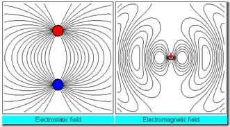
Example 1: A small dipole antenna.  Please refer to the following figure for the radiation wave.  It vividly shows how static electrical field becomes electromagnetic wave when the dipole is oscillating. 

 

Fig. 1: Electrostatic field and electromagnetic wave

Example 2: for a λ/2 dipole antenna, the radiation wave is shown in the following figure.  The maximal radiation wave is at equator.  No radiation wave at the north and south poles.

 

Fig. 2: λ/2 dipole antenna radiation wave

Example 3: for a λ wavelength dipole antenna, the radiation wave is shown in the link.  The maximal radiation wave is at equator.  Again, no radiation wave at the north and south poles.

 Example 4: for a 3λ/2 dipole antenna, the radiation wave is shown in the following figure.  The maximal radiation wave is 45 degree between the equator and two poles.  Again, no radiation wave at two poles.

 

 Fig. 3: 3λ/2 dipole antenna radiation wave

The above radiation wave animation is essentially derived from Maxwell equations.  The process is very cubersome and only solved by numerical method in computer.

Dipole Antenna Lumped Circuit Model

The core equivalent circuit of a dipole antenna is a serial RLC resonator.  Intuitively, the dipole antenna acts as an open circuit as a serial RLC resonator at low frequency as shown in Fig. 4(a).

On the contrary, the equivalent circuit model of a loop antenna is a parallel RLC resonator.  The loop antenna behalves as a short circuit as the parallel RLC resonator at low frequency as shown in Fig. 4(b).

The resonant resistance Rrad is not a physical resistance, but an equivalent resistance representing the radiative to the air.  Radiation resistance is only part of the antenna impedance.  Inductive and capacitive reactance are also present.  Energy that is transferred to the near field relates to the reactive component of the current in the antenna.  This is the 1/R^2 component of the electric and magnetic fields that we neglected when deriving the expressions for the far fields. 

A serial RLC resonator is only a first order approximation.  We need to consider other effects for a real antenna at RF frequency.

Fig. 4: Dipole and loop antenna equivalent circuit model

1. Rs, ohmic resistance and skin effect: a real antenna has finite ohmic resistance.   Rs also increases proportionally to sqrt(f) and becomes significant at high frequency.

2. Cp, parasitic capacitance of antenna. It can be modeled as a shunt capacitance.

Fig. 4(c) shows the equivalent circuit model including Rs and Cp, a better model than a serial RLC model.  We called it a lumped circuit model because we borrow circuit concepts (such as R, L, C, voltage, and current) to model the field behavior (such as electrical field, magnetic field, wave).  Strictly speaking, the lumped circuit model is only valid at low frequency where the wavelength is much longer than the antenna.  Nevertheless, we can break the entire operating freuqency range into different segment and use different lumped circuit model.

Lumped Circuit Model vs. Wavelength

When the dipole is very short (relative to wavelength), the dipole can be modeled as a series RLC circuit in which the impedance is dominated by radiation resistance and capacitive reactance. As the antenna is made longer, Rrad and XL increase and XC decreases. When the physical length equals λ/2 , XL = XC with a resulting impedance of Rrad (~73W).  As the antenna is made longer than λ/2, the model is a parallel RLC circuit. When length equals λ, the tank LC circuit has infinite impedance, leaving the parallel Rrad (~200W) as the net impedance.  Between a length of λ and 3λ/2 (Rrad~105W), the model is a series RLC circuit, and so forth.  This result is sumarized in Fig. 4(d).

See the figure for the variation in Rrad, which itself varies with wavelength.  Note that Rrad is about 73W at λ/2.   So we want to use a 75 ohm cable to match the impedance of a half-wave dipole in order to have maximum power transfer from the generator to the antenna. Notice that we used the impedance of space, ήo, in the calculation of Rrad. If we do not use a length of λ/2, there will be impedance mismatch and reflections, leading to a standing wave ratio greater than unity, i.e. less than maximum power transfer to the antenna.

Fig. 5: Dipole antenna radiation resisance vs. λ

Bandwidth
Note that the system is designed for specific frequency; i.e. at any other frequency it will not be one-half wavelength. The bandwidth of an antenna is the range of frequencies over which the antenna gives reasonable performance. One definition of reasonable performance is that the standing wave ratio is 2:1 or less at the bounds of the range of frequencies over which the antenna is to be used.

Dipole Antenna Smith Chart

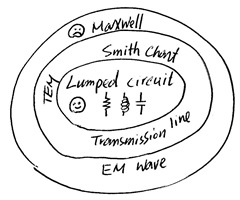
It seems that there is a delimma to get a full picture of a simple dipole antenna.  Solving Maxwell equations provides the accurate solution, but loses the physical intuition and not practical due to the computation complexity. 

Lumped circuit model provides a simple approximation of a dipole antenna, it is useful but only valid within limited frequency range.  The situation is shown in Fig. 6.

Fig. 6: Different abstration in electrical discipline

Luckily, there is a another tool originally derived from transmission line, namely Smith Chart, provides useful physical insight and enough accuracy for understanding the dipole antenna.  A brief introduction of Smith Chart is on the other article.  Lumped circuit is a subset included in Smith Chart.  Smith Chart (transmission line) is based on a specific EM wave called TEM (tranverse EM) wave where the dynamic electrical and magnetic fields are perpendicular to the wave propagation direction.  The majority of EM wave and waveguide either belong to the TEM domain or can be approximated by TEM wave.  That is, Smith Chart is a very useful tool to solve most electrical problems.

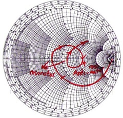
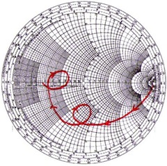
Fig. 7 shows the Smith chart of the input impedance (S11) of a monopole (half of a dipole antenna) without Rs and Cp.  The red trace starts from open circuit and capacitive at low frequency, and intersects at real axis at the first resonant frequency (λ/2, 36W).  The input impedance becomes inductive after the first resonance till it reaches the second resonant frequency (λ, 105W) so on and so forth.  Fig. 8 shows the Smith chart of a similar monopole antenna but with Rs and Cp.  Clearly, the input impedance is capacitive due to Cp at the first resonant frequency. 

Fig. 7: S11 of a monopole antenna without Rs and Cp

 

Fig. 8: S11 of a monopole antenna with Rs and Cp