Beauty of Dipole Antenna

Before diving into the dipole antenna, let's feel the simple beauty of radiation wave of a dipole antenna.  A good picture is worth a thousand words.

Example 1: A small dipole antenna.  Please refer to the following figure for the radiation wave.  It vividly shows how static electrical field becomes electromagnetic wave when the dipole is oscillating. 

 

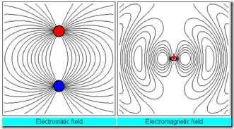
Fig. 1: Electrostatic field and electromagnetic wave

Example 2: for a λ/2 dipole antenna, the radiation wave is shown in the following figure.  The maximal radiation wave is at equator.  No radiation wave at the north and south poles.

 

Fig. 2: λ/2 dipole antenna radiation wave

Example 3: for a λ wavelength dipole antenna, the radiation wave is shown in the link.  The maximal radiation wave is at equator.  Again, no radiation wave at the north and south poles.

 Example 4: for a 3λ/2 dipole antenna, the radiation wave is shown in the following figure.  The maximal radiation wave is 45 degree between the equator and two poles.  Again, no radiation wave at two poles.

 

 Fig. 3: 3λ/2 dipole antenna radiation wave

The above radiation wave animation is essentially derived from Maxwell equations.  The process is very cubersome and only solved by numerical method in computer.

Dipole Antenna Lumped Circuit Model

The core equivalent circuit of a dipole antenna is a serial RLC resonator.  Intuitively, the dipole antenna acts as an open circuit as a serial RLC resonator at low frequency as shown in Fig. 4(a).

On the contrary, the equivalent circuit model of a loop antenna is a parallel RLC resonator.  The loop antenna behalves as a short circuit as the parallel RLC resonator at low frequency as shown in Fig. 4(b).

The resonant resistance Rrad is not a physical resistance, but an equivalent resistance representing the radiative to the air.  Radiation resistance is only part of the antenna impedance.  Inductive and capacitive reactance are also present.  Energy that is transferred to the near field relates to the reactive component of the current in the antenna.  This is the 1/R^2 component of the electric and magnetic fields that we neglected when deriving the expressions for the far fields. 

A serial RLC resonator is only a first order approximation.  We need to consider other effects for a real antenna at RF frequency.

Fig. 4: Dipole and loop antenna equivalent circuit model

1. Rs, ohmic resistance and skin effect: a real antenna has finite ohmic resistance.   Rs also increases proportionally to sqrt(f) and becomes significant at high frequency.

2. Cp, parasitic capacitance of antenna. It can be modeled as a shunt capacitance.

Fig. 4(c) shows the equivalent circuit model including Rs and Cp, a better model than a serial RLC model.  We called it a lumped circuit model because we borrow circuit concepts (such as R, L, C, voltage, and current) to model the field behavior (such as electrical field, magnetic field, wave).  Strictly speaking, the lumped circuit model is only valid at low frequency where the wavelength is much longer than the antenna.  Nevertheless, we can break the entire operating freuqency range into different segment and use different lumped circuit model.

Lumped Circuit Model vs. Wavelength

When the dipole is very short (relative to wavelength), the dipole can be modeled as a series RLC circuit in which the impedance is dominated by radiation resistance and capacitive reactance. As the antenna is made longer, Rrad and XL increase and XC decreases. When the physical length equals λ/2 , XL = XC with a resulting impedance of Rrad (~73W).  As the antenna is made longer than λ/2, the model is a parallel RLC circuit. When length equals λ, the tank LC circuit has infinite impedance, leaving the parallel Rrad (~200W) as the net impedance.  Between a length of λ and 3λ/2 (Rrad~105W), the model is a series RLC circuit, and so forth.  This result is sumarized in Fig. 4(d).

See the figure for the variation in Rrad, which itself varies with wavelength.  Note that Rrad is about 73W at λ/2.   So we want to use a 75 ohm cable to match the impedance of a half-wave dipole in order to have maximum power transfer from the generator to the antenna. Notice that we used the impedance of space, ήo, in the calculation of Rrad. If we do not use a length of λ/2, there will be impedance mismatch and reflections, leading to a standing wave ratio greater than unity, i.e. less than maximum power transfer to the antenna.

Fig. 5: Dipole antenna radiation resisance vs. λ

Bandwidth
Note that the system is designed for specific frequency; i.e. at any other frequency it will not be one-half wavelength. The bandwidth of an antenna is the range of frequencies over which the antenna gives reasonable performance. One definition of reasonable performance is that the standing wave ratio is 2:1 or less at the bounds of the range of frequencies over which the antenna is to be used.

Dipole Antenna Smith Chart

It seems that there is a delimma to get a full picture of a simple dipole antenna.  Solving Maxwell equations provides the accurate solution, but loses the physical intuition and not practical due to the computation complexity. 

Lumped circuit model provides a simple approximation of a dipole antenna, it is useful but only valid within limited frequency range.  The situation is shown in Fig. 6.

Fig. 6: Different abstration in electrical discipline

Luckily, there is a another tool originally derived from transmission line, namely Smith Chart, provides useful physical insight and enough accuracy for understanding the dipole antenna.  A brief introduction of Smith Chart is on the other article.  Lumped circuit is a subset included in Smith Chart.  Smith Chart (transmission line) is based on a specific EM wave called TEM (tranverse EM) wave where the dynamic electrical and magnetic fields are perpendicular to the wave propagation direction.  The majority of EM wave and waveguide either belong to the TEM domain or can be approximated by TEM wave.  That is, Smith Chart is a very useful tool to solve most electrical problems.

Fig. 7 shows the Smith chart of the input impedance (S11) of a monopole (half of a dipole antenna) without Rs and Cp.  The red trace starts from open circuit and capacitive at low frequency, and intersects at real axis at the first resonant frequency (λ/2, 36W).  The input impedance becomes inductive after the first resonance till it reaches the second resonant frequency (λ, 105W) so on and so forth.  Fig. 8 shows the Smith chart of a similar monopole antenna but with Rs and Cp.  Clearly, the input impedance is capacitive due to Cp at the first resonant frequency. 

Fig. 7: S11 of a monopole antenna without Rs and Cp

 

Fig. 8: S11 of a monopole antenna with Rs and Cp