Steady State Kalman Filter

Time Varying or Stationary?

一般而言 Kalman filter 是 time varying 的 filter.  多數 Kalman filter 的應用也是 time varying system, 例如 navigation, gesture recognition, etc.  

另一類的應用: 如果 A, B, Bw, C, (參考 Berkeley article) matrices and (A, C) is observable or detectable; (A, Bw) is controllable or stabilizable. 

同時 covariance matrices Q, R 是 stationary and semi-positive definite.  Kalman filter 有 steady state 的 solution.  

Steady state 的參數包含:

• state mean, x(k) -> x,  or m(k) -> m (only one)
• state covariance 有兩個:  P+ 是 prediction step 之後的 covariance;  P- 是 update step 之後的 covariance.

        P+ > P-;   P+ = A' P- A + Q

       or P- = A'.inv (P+ - Q) A.inv

• Kalman gain (only one)

 

Method A:  Brute force iterative simulation

Method B:  P = P

Method C:  discrete algebraic Ricartti Equation (DARE) steady state equation 如下:

(可以參考 const_v.py code for simulation example)

 

ARE

RE: Riccarti Equation    ARE: (Algebraic Riccarti Equation)

Stanford EE363 note

 

 

Another Berkeley article

Ms 是 prediction step 之後的 covariance.  

Fs 是 steady state 時的 Kalman Gain!!!

 

Example1:  DC offset estimation: A=C=1 ; Bw=1  

P+ = P- +Q

P+ = P+ + Q - P+ ( P+ + R)^-1 P+

P+ + R = P+^2 / Q

P+ = 0.5 * (Q + sqrt(Q^2 + 4QR))  as expected

  

Example 2:  Constant Velocity Model: A = [1, 1; 0, 1] , C =[1, 0],  Bw=1, V=R, W=[qo, q1; q1, q2]

case 1:  W = [q0, 0; 0, 0]  process noise only on position, reduce to example 1??  Q = q0

case 2:  W = ?? process noise only on velocity ->?

 

 

古典力學

 

三種不同的古典力學詮釋

Newtonian   

Lagrangian

Hamiltonian

 

Newtonian (牛頓力學)

Newtonian 的變數是 F, x, x_dot, x_dot_dot; 2nd order differential equation

Newtonian 哲學是力造成速度的變化，正比於加速度

Pro:  1. 可以處理 non-conservative force (非保守場之力); 如摩擦力

         2. 比較直覺

Con: 1. 力很難分析 (vector 而非 scaler; 有方向性)

         2. 不同座標的 transformation 更複雜

Lagrangian

 

Lagrangian 的變數是 q and q_dot; 2nd order differential equation

 

Lagrangian 哲學是數小作用力原理

 

Pro:   1. L = T - U ; scaler only, no vector.  Or use Newtonian to derive L.

          2. General coordinates 

 

Con: 1. 只處理 conservative force (保守場之力)

 

       

Hamiltonian

Hamiltonian 的變數是 p and q; 1nd order differential equation

Hamiltonian 哲學是 reversibility -> phase diagram -> fluid/flow Lioville equation

-> field theory 

Pro:   1. H = Pq - L ; scaler only, no vector.

          2. General coordinates 

          3. pq are symmetry

          4. direct link to Quantum mechanics

 Con: 1. 只處理 conservative force (保守場之力)

 

 

Parameter Estimation – Cramer Rao Lower Bound

在 estimation theory 中，時常用到的 bound 是 Cramer-Rao Lower Bound, 簡稱 CRLB or CRB.

CRLB 的重要性在於 (i) 這個 lower bound 對不同的 estimators 能做的多好有一個比較的依據; (ii) 更重要的是 CRLB  常常是可以達到的 (也許在某一些條件下如 high SNR or asymptotically).  不像有一些數學上的 bound 只是好看而已。

Some Uses of CRLB

之後再補

What is CRLB?

CRLB is a lower bound on the variance of any unbiased parameter estimator:

所以到底 CRLB 為什麼存在以及如何定義?

Score, MLE, Fisher Information, CRLB

如何定義如下:

First, we define log likelihood function  LLF = ln{LF} = ln { p(x;q) } where p(x;q) is the pdf of x, or likelihood function of q.

V 稱為 score, 代表 LLF 的 first derivative, 也是 LF 的 sensitivity.

記得 ML estimator: q_hat 滿足 d(LLF)/dq = V = 0 代表找 LF or LLF 的最大值

事實上, ML estimator asymptotically achieves the Fisher information (and the CRLB) in the limit.

另外 under certain regularity condition, the first moment of V (即 expected value) is 0 .

The second moment of V is named Fisher Information (always > 0)

再回到 CRLB:  直覺來說，若是 LLF vs. q 很集中，estimation 的效果會比較好，Fisher Information (FI) 比較大，CRLB 就會比較小。相反如果 LLF vs. q 很平緩，FI 比較小，CRLB 就會比較大。 衡量集中或平緩的特性就是曲率，粗略來說，CRLB 的定義就是 LLF 曲率的倒數 * –1 (x-1 是轉正值).

注意 variance 大，FI 比較小。這和 Shannon Information (Entropy) 的定義相反。FI 是從估計的角度出發，variance 小則估計準，information 比較多。Shannon Information 是從 surprise 的角度出發，variance 小則沒有 surprise, information 比較少。

上述的第一項是 0 after E{}.   Therefore, the E{curvature (*-1)} is the same as Fisher information

CRLB = 1/(Fisher Inforamtion)

因此曲率大的  LLF 的 information 比較多，或是 CRLB 比較小。Estimator 有機會做的比較準確。

 

另一個 CRLB 有關的定理

 

CRLB 例子

Example 1: DC + AWGN

x[n] = A + w[n]      n = 0, 1, …, N-1

LLF function is as follows:

First derivative:  V = d(ln p)/dA = 1/sig^2 sum(x[n] – A)  

ML estimator:  A_hat =  1/N sum(x[n])

Second derivative:  d^2(ln p)/d^2 A = –N/sig^2

Fisher Information  I(A) = N / sig^2

CRLB = sig^2/N

ML estimator 和 MMSE estimator 相同，同時都可以達成 CRLB!

 

Example 2: Sine Wave + AWGN (only unknow is phase)

fo < 1/2 is to keep below Nyquist sampling frequency.

First, the pdf or likelihood function.  This is a general function even when A, fo, and phi are all unknown.

 

Assuming the only unknown is phase,

 

 

The ML estimator looks very complicated (V=0) and no close-form (I think).   The efficient estimator does NOT exist based on the aforementioned theory.

Example 3: Complex Sine Wave + AWGN (amplitude, frequency, and  phase are unknowns)

If amplitude is unknown, 結果和 DC+AWGN 一樣。唯一的差別是 A –> A cos(.), 如果 N 夠大，A^2 –> A^2/2.   The CRLB doubles.

How about if both amplitude and phase are unknow?  It can be shown that amplitude and phase are orthorgonal.  Therefore,  the amplitude and phase estimation CRLB bound can be treated separately.

A more general CRLB with amplitude, frequency, and phase are unknown can be found in D.C. Rife’s paper.   

First, we consider the complex sine wave case, i.e. the sine wave contains both cos and sin.

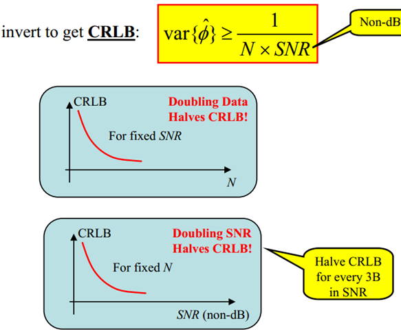
可以看到 amplitude and phase 的 Fisher information 分別為 N/sig^2 and N*bo^2/sig^2.  這和之前的結論一致。amplitude 只和 sig^2 and N 有關；phase 和 SNR and N 有關。但是 complex sine wave 的 CRLB 比 sine wave only CRLB 小一半。

如果 frequency 也加入就更有趣。amplitude and phase 正交；amplitude and frequency 正交；但是 frequency and phase 非正交。直覺上 make sense, since frequency is phase derivative.  從 eq. (13) 也可以看出。J12=J21 <> 0

Complex sine wave (includes both sin and cos) 結論如下:

Amplitude 和 frequency and phase 正交，所以 eq.(18) hold for all cases.  eq.(19) 如上述討論 (frequency is known).  對於 frequency and phase all unknown 的情況最複雜。Basically, amplitude CRLB is proportional to sig^2/N; phase CRLB is proportional to 1/(SNR*N)); frequency is proportional to Fs^2/(SNR*N^3).  Note that N = T * Fs (?)

Example 4: Real Sine Wave + AWGN (amplitude, frequency, and phase are unknowns)

Next, we consider only real sine wave. 

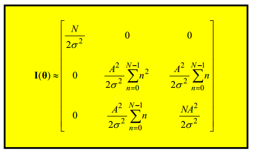
The Fisher Information Matrix (FIM) is shown below:

Compared with the complex sine wave FIM, some second order items are ignored for simplicity (when N is large). 

The CRLB of real sine wave is very similiar to the complex sine wave.

Example 3 and 4 seems to imply that estimate frequency (1/N^3) is a lot more accurate than phase (1/N)!

下面的例子 Example 4 中的 method 3 and 4 似乎利用這個特性假設 perfect frequency estimation.

 

Example 5: Comlex Sine Wave with frequency offset and IQ imbalance (amplitude, frequency, and phase are unknowns)

Problem statement: A cos(wt + q) + j B sin(wt + q + f) + w(t) + j w’(t)   Estimate amplitude mismach (A/B) and phase mismatch f.  

The following method 1/2/3 employ a sine wave test tone (as a LIF) and estimate the amplitude and phase mismatch.   

Method 4 uses received preamble containing a known pilot sequence directly and a ZIF receiver to estimate the amplitude and phase mismatch assuming ideal frequency estimation and

Method 1: Separte estimate: A cos(wt + q)+w(t) and  B sin(wt + q + f)+w’(t)

var(A) > 2 sig^2/N   var(B) > 2 sig^2/N    var(A-B) > 4 sig^2/N

1. var(q) > 4/(SNR*N)    var(q + f) > 4/(SNR*N)     var(f) > 8/(SNR*N)  (?)

 

Method 2: Cross correlation of I1’ and Q1’ 如下圖, then

LPF{(Acos(wt + q)+w(t))(Bsin(wt + q + f)+w’(t))} = AB/2[sin(f)]+Bw(t)sin()+Aw’(t)cos()+w(t)w’(t)

where LPF is simply a summation.

Therefore, it becomes DC + AWGN  (DC = AB/2 sin(f)   AWGN ~ Bw*sin+Aw’cos+w*w’)!  

var(sin(f)) ~ var(f) > 2*sig^2/NAB=2/(N*SNR)    (w*w’ is zero mean, but not Gaussian!)

這時的 CRLB 比較小，同時也不需要 estimate frequency!  How to estimate A/B? same as method 1? or square I and Q then average?

Method 3: Extension of method 2.

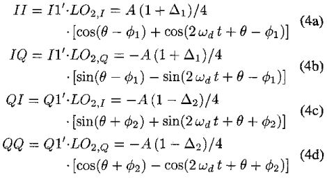
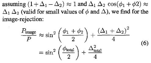
接下來假設 wd 可以準確 estimate, 以及在 digital domain 可以 create 90度 perfect 的 cos(wd) and sin(wd).  可以得到 II, IQ, QI, QQ.  這和 method 2 不同。method 2 直接 I1’ * Q1’, 因此不需要 estimate wd. 

 

How to derive the CRB? Wait for next time.  The result should be simiar to the next method 4.

 

Method 4: Let’s assume rRF(t) is a general received signal with preamble containing a known pilot sequence (instead of test tone).  Please refer this article.

where fd = fo - flo

Assuming ideal frequency estimation (fd = 0!?), g(t) is a match filter, and ideal timing recovery (?),  then

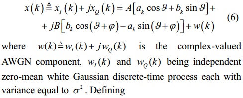
因此問題變成 given ak, bk, xi, and xq, estimate A, B, q, and f.  一旦 estimate 出 A, B, q, and f,

簡單來說，就是先用 preamble 中 known pilot sequency to estimate amplitude mismatch (A/B), phase mismatch(f), and phase offset (q).  再來用 eq (10) corrects mismatch and phase offset.  The CRLB is shown as follows:

Es/No = 1/sig^2   CRB(q) = 1/N*SNR   CRB(f) = 2/N*SNR  CRB(A)=CRB(B)=sig^2/N

 

Example 6: how about non-sine,  eye diagram?  harmonic estimation?  very low frequency (close to DC; or Nyquist)?

ML Estimation and MAP Estimation 差異

剛才看了 BAYESIAN ESTIMATION,   這篇文章把 MAP, ML, MMSE, MAVE 解釋和比較的很清楚 under the Bayesian estimation framework.  可以直接參考跳過本文。(Chap4 of “Advanced Digital Signal Processing and Noise Reduction”, Second Edition. by Saeed V. Vaseghi)

ML (Maximum Likelihood) and MAP (Maximum A posteriori Probability) estimation/detection 非常類似，也容易混淆。其實只有一點差異。

(2.1) 是 MAP detection;  (2.3) 是 ML detection.   MAP 和 ML 之間的關係是 (2.2) (Bayes theory). 

簡單來說，ML (eq. 2.3) 和 s 出現什麼的機率無關 P(s was sent).  意即完全不考慮 s 的 pdf; 或者假設所有的 s 有相同的機率。在這情況下，eq. 2.2 and eq. 2.3 are equivalent; ML estimation 等同 MAP estimation.  (P(v is observed) is a constant in eq. 2.2).

In summary,  ML (or MLE) 和 MAP estimator 的關係可以更簡化如下。唯一的差別就是 MAP 多乘了 theta 的  distribution.

 

舉例而言，s=+1 or –1 is a simple Bernoulli distribution. 

P(s=+1)=p  P(s=-1)=1-p=q           n ~ N(0, sig^2)

ML estimator:  s* = arg max P(v is observed | s was sent)

MAP estimator: s* = arg max P(v is observed | s was sent) * P(s was sent)

兩者的差異如下圖:

ML estimator:  v>0  s*=+1;  v<0  s*=-1   regardless p

MAP estimator: v>a  s*=+1;  v<a s*=-1   a depends on p (can be computed numerically)

如果 p=0.5,  a=0 and equivalent to ML estimator.  如果 p>0.5, a 就是負值，  s*=+1 的區間變大，反之亦然。直覺來說，p>0.5 代表 P(s=+1) 的機率比較大，因此在 estimate 時，比較 favor s=+1, 也就是 threshold a<0.