力耶？勢耶？孰優孰劣

孫子兵法：故善戰者，求之於勢。善戰人之勢，如轉圓石於千仞之山者，勢也。故上兵伐謀，其次伐交，其次伐兵，其下攻城。伐謀、伐交就是造勢、借勢。伐兵、攻城就是以力取勝。孫子兵法明顯認為 "勢" 優 "力" 劣。

古典力學的兩種 approach

一是大家都熟悉的牛頓力學 (Newtonian mechanics) 和三大定律 (實際上是假設)：即 (i) F=0 的慣性定律, (ii) F=mA 運動定律,  和 (iii) 作用力和反作用力定律。其中最重要最關鍵的物理量就是力。這也是為什麼 mechanics 中文翻譯為 "力" 學。

另一類 approach 是基於最小作用原理 (least action principle)，通常稱為 Lagrangian mechanics 或是 Hamiltonian mechanics。這裹只有一個假設，就是運動的物體會遵循最小的 action。什麼是 action(S)，可以用下面公式定義：

 

其中 L = T - V。T (kinetic energy) 是動能。V (potential) 通常稱為位能，或是勢(能)。雖然 V 大多是位置的函數，但也可能是速度或是時間的函數，所以位能不是妥當的翻譯。

只要能找出 L (i.e. T-V)，其它只是計算。T=1/2mv2 是 well-known.  主要的工作就是找出 V (勢)。

簡言之：牛頓力學 (Newtonian mechanics) 主要的工作就是找到所有的力。Largrangian or Hamiltonian mechanics 主要的工作就是找到勢。在多數的情況，找勢比找力簡單容易。意即"勢" 優 "力" 劣。

靜力學的例子

考慮一條均勻繩子或鏈子兩端固立，在重力場中自然垂下如下。

從牛頓力學的靜力學觀點而言，每一小段鏈子的重力和上下兩端的張力的合力為零。雖然不難，但須費一番功夫。

在靜力場中，動能 T=0, S = (t2-t1) V.   因此在靜力學中，最小作用力原理簡化為最低勢能原理。解法如下：

因為重力場函數是 -gy, 所以只要將每一小段鏈子質量乘上重力場即是每一小段的勢。最後再把所有小段的勢積分就得到全部的勢。

最小作用力原理的優點

(A) 不用找力，不論是明顯的外力 (重力)，或是不明顯的內力 (張力)；只需要找勢。勢通常只由外力造成，內力可以被忽略(除非有彈力位能)。這讓思考簡化很多，也容易讓電腦自動計算。

(B) 同時勢能是一純量，而力是一向量。這也讓計算簡化許多。

(C) 除此之外，最小作用原理是一普遍的原理。可以同樣適用在相對論力學，量子力學上。這是比牛頓的力學三定律更基本的原理。此外，結合廣義座標和微分幾何，可以得到更深的物理意義。請參閱參考資料。

參考資料: "The Variational Principles of Mechanics" by Lanczos

LDO Regulator 設計要點

LDO 設計最主要的工作是設計 PMOS, error amplifer, 和適當的 frequency compenstation 電路，步驟如下：

Step 1: 由 steady state 決定 PMOS 的大小。主要是由 Iload 和 PMOS 的 Vdrop (droupout voltage) 決定，條件是讓 PMOS 維持在 saturation.

以 Iload = 50mA and Vdrop = 200mV 為例, 假設為 0.35um 3.3V 製程 uCox = 65uA/V^2.    W/L ~> 40,000. 

For L = 0.4um (3.3V device), W > 16mm,

WL = 6400 um^2  or 80 um x 80 um area.   The gate capacitance is around 80 um x 80 um x 6 fF = 38.4 pF.

 

Step 2: 由 transient condition 決定 close loop (包含 error amplifier and output PMOS) 的頻寬 BW 和 Cload 的大小。

DVdrop(X) 是指在 x 點 (output point) 當 Iload 由0 跳升為 Iload 時的 voltage drop。這是由三部份所組成，ESR, ESL, and C1 的壓降。如果 ESL 很小且 Iload 不大，可忽略 ESL 的壓降。一般我們希望 DVdrop 控制在 Vout 的+/-10% 之內。因此，BW* Cload 必須大於一個常數。

 

 

 

( Cload * BW > constant )

 

先選 output cap 的大小。

Q = CV   i = C dv/dt

dv  = i * ESR +  i / C * dt

i –>  current;  C –> output cap

dt –> close loop bandwidth dt * BW = 0.35  -> dt = 0.35 / BW

dv = i * ESR + 0.35 * i /  (C * BW)

example:  這是由 time domain 決定。 for example, 1.2V 10% is  120mV.   output current is 60mA. ESR = 0.5Ohm, vdrop = 30mV.  dv = 90mv = 0.35*i / (c * BW)   (c*BW) > 0.23

opamp 的 BW = 100KHz  c > 3uF.  

 

Step 3: 決定 frequency compensation 的方式

一般使用 single stage opamp 以簡化 frequency compensation 方式。因此 output pole can be obtain by  Rpar * C par.  Gain can be obtain gm * Rpar.  Therefore, the transfer function is gm * Rpar / (1 + Rpar * Cpar * s).    At high frequency, the UGF = gm / Cpar.  (gm usually around 400uA/V, therefore 10M rad or 1.5MHz. 

On the other hand, the output has another dominant pole, usually Gp = gmp * Rout;  Cout * Rout, therefore, the UGF of output pole is gmp / Cout.  assume gmp = 100mA/V, Cout = 10uF, UGF = 10K rad or 1.5kHz, far smaller compared with originally ucf. 

如上所述，若沒有 compensation, 兩個 low frequency poles 會造成 no phase margin.  常見解決方法是在 output cap 上加一個 ESR zero,  但仍有其他的 output pole (usually needs to be less than 10% of output cap, Pb), 如下圖所示 。

 

 

然而 ESR 所造成的 zero, 必須小心控制，太小或太大都不合適。太大乍看之下很好，甚至可以讓 zero 和 Pa 互消，但間題是 ucf 太高， 會被下一個 pole 造成 low phase margin.  相反的，如果 ESR 太小，對 phase margin 沒有什麼貢獻。

LDO Regulator 簡介

LDO (Low Dropout Regulator) 的主要功能就是在輸入電壓 (Vin) 或是輸出電流 (Iout) 變動的情形下，仍然維持穩定的輸出電壓 (Vout)。如上圖所示，如果 Vin (就是 line) 有一個電壓的突升, 輸出電壓 Vout 也會隨之改變，但經由 LDO 的回授電路會把 Vout 穩定在原來的電壓，因此 Vout 有一些電壓漣波，同時最終穩定的電壓也有些許的變化。Vout 對 Vin 的變化稱之為 line regulation，後面有更詳細的說明。同樣的如果輸出電流突升，輸出電壓 Vout 也會改變， Vout 對 Iout 的變化則稱為 load regulation。

 

上圖是一個 LDO 的原理圖，主要有四個部份。簡單卻包含了類比電路的feedback 控制、和補償的原理。

Reference 和 RC filter: 通常為 bandgap 電路加上 RC 濾波電路提供穩定的參考電壓。

Error Amplifier 及 R1/R2 分壓: 通常為一簡單的 opamp 放大輸出電壓(經R1/R2 比例)和參考電壓的誤差。注意此處參考電壓接正極。實務上 Pass FET 多為 PMOS 提供多一次反向。因此參考電壓會接負極而非正極。

Pass FET: 一般為一個巨大的 PMOS。PMOS 的大小由提供的電流和 dropout voltage 決定。

Cout 及 Rload: Cout 為輸出濾波及提供快速電流給 output load。可以用 Rload 模擬 LDO 提供的電流。 Cout 通常會有寄生電感和電阻，稱之為 ESL 和 ESR (equivlaent serial resistance)。其中 ESR 對於 LDO 的穩定(或振盪)相當重要。

 

LDO performance: AC and Step Response

LDO 常見的特性包含 frequency domain PSRR 和 time domain step response。以 Vin 的 PSRR 為例：

 

上圖為 Vout 對 Vin 在不同頻率正弦波的 rejection ratio 。一般可分為三區：

• Region 1 是由 reference 和 RC filter 決定。由於 RC 面積的限制，一般 RC filter 的頻率很難低於100 Hz。
• Region 2 是由全部的 feedback loop 的 gain 和 frequency response 決定，包含 error amp, pass FET, output load 和 R1/R2。一般 dominant pole 是由 Cout Rload 決定 (10uF, 10 Ohm ~  1.5kHz)。
• Region 3 是由 output 電容分壓決定。Cout 愈大，PSRR 在 region 3 愈高。

 

再以 load current 的 500mA step response 為例：

 

可分為二區

第一區為高頻區 (以 close loop 的 loop bandwidth 為準)。因為 error amplifier 和 PMOS 來不及反應，電流由外接電容供應，因此 Vout 往下降。可以根據 output cap 以及寄生的電阻電感、再細分為三個部份壓降，分別為 ESR, 其次為 ESL, 然後是 cap 造成。ESL 壓降最快，反應電流的變率(微分)；ESR 壓降其次，直接反應電流； cap 壓降最慢，反應電流的積分 (droop)。

一旦進入了 loop bandwidth 的反應時間，error amplifier 和 PMOS 開始動作，加大的電流同時供應 output load 以及對電容充電。電壓上升，這時對應的是 PSRR 的 region II 。

理論上可以同樣得出 Vin  的 step response 和 load current 的 ac response。可由 fourier transform 得到。不過一般 LDO 較少用到。

	AC response	Step response
Input Voltage	PSRR, 週期性 noise	step noise
Load current	很少用到	常見且重要

 

LDO Frequency Compensation

上述的 LDO 很明顯有 stability 的問題，因為有兩個低頻的 poles：一個位於 output 的 dominant pole，由 Cload (~10uF) 所造成；另一個位於 PMOS  gate 的 non-dominant pole，由 PMOS 的 gate capacitance (Cgate ~ 幾十 pF) 所造成。另外加上一些高頻的 poles, 會讓 phase margin 小於10度而引起 stability 的問題。

更麻煩的是 Cload 所看到的等效電阻會隨著 Iload 有很大的改變。大電流時 (50-100mA) 等效電阻小 (Rload 和Rpar, 幾十歐姆)，小電流時 (<1mA) 時等效電阻大 (> kOhm)。會造成 dominant pole 頻率可能相差百倍。

相反的，Cgate 所看到的等效電阻 (error amplifier output impedance) 卻是與 Iload 無關，non-dominant pole 的頻率基本上不會隨著 Iload 改變 (但仍與 PVT 有關)。因些有可能藉著增加 zero 來補償 (或者可想成 cancel) non-dominant pole 而增加 phase margin。

 

最容易加上 zero 的方法就是直接利用 output cap 上的 ESR，自動創造出一個位於 Cload* ESR 的 zero。這個增加 zero 的方法簡單有效，廣為 LDO 所用，但是有一些限制。

1. 為了能適當的補償或 cancel non-dominant pole，ESR 值有一定的範圍，太大或太小都會造成問題。
2. 必須選擇 tantalum (鉭質)電容，因為 ESR 值適中 (~100 mOhm) 且不隨著溫度變化太大。ceramic 電容雖然體積小且低價，但 ESR 過小 (<10 mOhm) 不適合。一般電解電容的 ESR 隨溫度變化太大也不適合。
3. 另外 ESR 在 Iload 變化時，會有額外的壓降而造成 Vout 上的 noise。

對於 LDO 更詳細的介紹請參考 LDO 設計重點一文。

藍牙簡介

如前文所述，bluetooth 己成為 mobile computing 的 de facto 外接的標準。本文主要討論 bluetooth 的規格及應用。

Bluetooth 有內定的 profile 決定有關的應用，可參考 wiki。以下舉出手機中常見的 profile:

• Hands Free and Headset profile: HFP / HSP
• Advanced Audio Distribution (Stereo) profile: A2DP
• Audio/Video Remote control profile: AVRCP

不同的 profile 並不完全是獨立的，常常是互相關連，如下圖所示。GAP 是最基本的 profile；GAVDP 是架構在GAP之上； A2DP 又是架構在 GAVDP之上。

以下說明各種 os/device 對 profile 的支援程度。以 embedded OS 而言，symbian 目前有最完整的 bluetooth profile 支援。

 

General OS

Windows XP SP2/Vista/7

The Microsoft Windows Bluetooth stack only supports external or integrated Bluetooth dongles attached through USB. It does not support Bluetooth radio connections over PCI, I²C, serial, PC Card or other interfaces.

Windows XP includes a built-in Bluetooth stack starting with the Service Pack 2 update, released on 2004-08-06.

The Windows XP and Windows Vista Bluetooth stack supports the following Bluetooth profiles natively: SPP, DUN, HID, HCRP.  Windows 7 also supports audio related profiles-HFP, HSP, A2DP and AVRCP natively.

 

Linux

The Linux operating system currently has two widespread Bluetooth stack implementations:

• BlueZ, included with the official Linux kernel distributions, initially developed by Qualcomm.
• Affix, developed by Nokia Research Center.

BlueZ is the official Bluetooth stack for Linux and is used in Google's Android OS. Its goal is to make an implementation of the Bluetooth wireless standards specifications for Linux. As of 2006, the BlueZ stack supports all core Bluetooth protocols and layers.  It was initially developed by Qualcomm, and is available for Linux kernel versions 2.4.6 and up.

 

MAC OS

Mac OS X: As of version 10.5, Mac OS X includes native support for A2DP on Bluetooth equipped Macs.  Version 10.4 does not support A2DP, but can be hacked to enable limited functionality.  Softick Audio Gateway for Mac OS X also supports A2DP. Despite being capable of A2DP, the iPhone variant of OS X provides no A2DP support as of October 2008. (But will be supported in future versions of the iPhone OS.)

 

Embedded OS

BlueMagic

BlueMagic 3.0 is Open Interface's (now Qualcomm) highly portable embedded Bluetooth protocol stack which power's Apple's iPhone and Qualcomm-powered devices such as the Motorola RAZR. BlueMagic also ships in products by Logitech, Samsung, LG, Sharp, Sagem, and more. BlueMagic 3.0 was the first fully certified (all protocols and profiles) Bluetooth protocol stack at the 1.1 level.

 

BlueCore Host Software (BCHS)

CSR's BCHS or BlueCore™ Host Software provides the upper layers of the Bluetooth® protocol stack (above HCI, or optionally RFCOMM) - plus a large library of Profiles - providing a complete system software solution for embedded BlueCore applications. BCHS supports 1.2, 2.0+EDR and 2.1+EDR. Current qualified Profiles available with BCHS: A2DP,AVRCP,PBAP,BIP,BPP,CTP,DUN,FAX,FM API,FTP GAP,GAVDP,GOEP,HCRP,Headset,HF1.5,HID,ICP,JSR82,LAP Message Access Profile,OPP,PAN,SAP,SDAP,SPP,SYNC,SYNC ML.

 

Windows CE/Mobile

Windows CE is Microsoft's embedded operating system, which also supports Bluetooth. However, different stacks can be installed on windows CE devices, including Microsoft, Widcomm, and Toshiba, depending on the embedded device on which the OS is installed.

Windows Mobile (previously Pocket PC, PPC): Version 5.0 and newer (with AKU 2.0), thus far based on the Windows CE 5.0 kernel, fully support A2DP if an appropriate device is present.

There is a huge amount of debate on the forums as to what Bluetooth profiles Windows Mobile devices support.  Below is the list that we support natively in the Microsoft Stack in AKU 2.0 of Windows Mobile 5.0 and beyond:

Generic Access Profile (GAP)
Generic Object Exchange Profile (GEOP)
Serial Port Profile (SPP)
Dial-up Networking (DUN) Profile
Hands-Free Profile (HFP)
Headset Profile (HSP)
Human Interface Device (HID) Profile
Object Push Profile (OPP)
ActiveSync-Over-Bluetooth
Advanced Audio Distribution Profile (A2DP)
Audio/Video Remote Control Profile (AVRCP)

The confusion typically starts because it is up to to the OEM to choose which ones they implement or to add additional support for other profiles.

 

Symbian OS bluetooth profile (v9.2)

Symbian OS is an operating system for mobile phones, which includes a bluetooth stack. All phones based on Nokia's S60 platform and Sony Ericsson/Motorola's UIQ platform use this stack. The Symbian bluetooth stack runs in user mode rather than kernel mode, and has public APIs for L2CAP, RFCOMM, SDP, AVRCP, etc. Profiles supported in the OS include GAP, OBEX, SPP, AVRCP, GAVDP, PAN, PBAP.  Additional profiles supported in the OS + S60 platform combination include A2DP, HSP, HFP1.5, FTP, OPP, BIP, DUN, SIM access, device ID.

There are two kinds of profiles provided for by Symbian OS: implemented and supported. Implemented profiles can be used directly from the existing components. When a profile is supported the licensee will need to provide its own APIs to make the functionality of that profile available to application developers.

The above figure shows the dependencies of profiles. The shaded profiles are implemented by the Symbian OS Bluetooth subsystem.

Implemented Bluetooth profiles

The following profiles are implemented by Symbian OS Bluetooth:

• Generic Access Profile (GAP)

• Serial Port Profile (SPP)

• Generic Object Exchange Profile (GOEP)

• Personal Area Networking (PAN) Profile

• Audio Video Remote Control Profile (AVRCP)

• Generic Audio Video Distribution Profile (GAVDP)

 

Android (Cupcake)

Android bluetooth is based on BlueZ on Linux.  New kernel based on Linux 2.6.27.  However, the bluetooth API is not supported till v1.0 release.  Google promised it will support A2DP profile.  The tentative release cupcake supports A2DP and AVRCP profiles.

iphone OS

iphone OS is based on MAC OS X.  The only bluetooth device opens now is the bluetooth headset.  It is annoying!

50/75 Ohm for RF?

所有 RF 工程師都熟悉如下圖 50 Ohm 的阻抗匹配。舉凡 LNA, PA, 天線, 高頻頭 (tuner), waveguide 等等，都要求 50ohm 的阻抗。唯一的例外是有線電視，通常使用 75ohm 的纜線。到底當初為什麼會選擇 50 或 75ohm的阻抗？以及在 rf ic 的設計上是否應沿用 50ohm 的阻抗？本文參考 Tom Lee 的說明給予一些解釋。

為什麼要做阻抗匹配?

常見的幾種說法：

1. Max power delivery：當阻抗匹配時，能傳遞最大的能量（功率）

2. 相反的，如果沒有適當的阻抗匹配，發射端的能量會反射，有可能損壞機器，如上圖的 phase array radar 系統所示。或者接收端可能收不到訊號。

為什麼用 50 Ohm 做阻抗?

主要有兩個考量：

1. Power delivery (能量傳遞):  主要考慮發射端能把最大的能量傳遞至天線或雷達。由於能量和阻抗成反比，阻抗愈小，電流愈大，能量愈大。

2. Power Attenuation (能量衰減): 所有的 wavegude 和 cable 都有雜散電阻。特別高頻有所謂的 skin effect, 會使電阻隨頻率(平方根)增加，因而讓發射或接收信號衰減。因此會希望阻抗愈大，電流愈小，損失的能量愈小。

同樣的考量也存在電力網上。電力網的解決之道是用變動的阻抗(變動的電壓和電流)來解決。在頭端和末端使用低電阻和高電流(110V/220V 電壓)以達到高能量傳遞。但在傳送過程中使用高電壓和低電流以避免能量衰減，同時維持高的能量傳遞。在 RF 中一般傳送的距離很短，也有相當的困難使用變動的阻抗。因此仍然以固定阻抗為主。

Tom Lee 的書花了一番功夫推導兩者的最佳值。就 power delivery 而言，最好的值是是 32 Ohm.  就 power attenuation 而言，最佳值約為 77 Ohm.  因此取平均值為 50 Ohm.  詳細的推導可參閱 Tom Lee 的書。然而在 cable TV 的應用，因為主要為通訊目的而選為 75 Ohm 以增加傳送距離。

RF IC 也應用 50 Ohm 做阻抗嗎?

當然是否定。因為 50 Ohm 或 75 Ohm 只是人為的選擇。以 RF IC 而言，既不能 power delivery 也非 power attenuation, 反而是重在 RF signal 的放大，frequency translation, filtering, etc. 除了和 IO interface 有關的電路仍應用 50 Ohm 以和外部元件匹配 (trace, 天線, etc.)，內部線路可用類似電力線做法用 variable impedance 以達成最佳的效果。甚至可以忽視阻抗匹配，因為非常短距離。例如 Ro 用低阻抗而下級 Ri 用高阻抗，如同設計低頻電路一樣。

數值方面的解釋可以參考 Crawford 的文章。

Beauty of Dipole Antenna

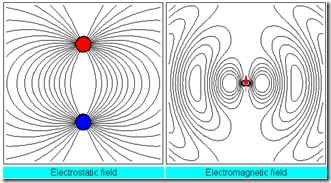
Before diving into the dipole antenna, let's feel the simple beauty of radiation wave of a dipole antenna.  A good picture is worth a thousand words.

Example 1: A small dipole antenna.  Please refer to the following figure for the radiation wave.  It vividly shows how static electrical field becomes electromagnetic wave when the dipole is oscillating. 

 

Fig. 1: Electrostatic field and electromagnetic wave

Example 2: for a λ/2 dipole antenna, the radiation wave is shown in the following figure.  The maximal radiation wave is at equator.  No radiation wave at the north and south poles.

 

Fig. 2: λ/2 dipole antenna radiation wave

Example 3: for a λ wavelength dipole antenna, the radiation wave is shown in the link.  The maximal radiation wave is at equator.  Again, no radiation wave at the north and south poles.

 Example 4: for a 3λ/2 dipole antenna, the radiation wave is shown in the following figure.  The maximal radiation wave is 45 degree between the equator and two poles.  Again, no radiation wave at two poles.

 

 Fig. 3: 3λ/2 dipole antenna radiation wave

The above radiation wave animation is essentially derived from Maxwell equations.  The process is very cubersome and only solved by numerical method in computer.

Dipole Antenna Lumped Circuit Model

The core equivalent circuit of a dipole antenna is a serial RLC resonator.  Intuitively, the dipole antenna acts as an open circuit as a serial RLC resonator at low frequency as shown in Fig. 4(a).

On the contrary, the equivalent circuit model of a loop antenna is a parallel RLC resonator.  The loop antenna behalves as a short circuit as the parallel RLC resonator at low frequency as shown in Fig. 4(b).

The resonant resistance Rrad is not a physical resistance, but an equivalent resistance representing the radiative to the air.  Radiation resistance is only part of the antenna impedance.  Inductive and capacitive reactance are also present.  Energy that is transferred to the near field relates to the reactive component of the current in the antenna.  This is the 1/R^2 component of the electric and magnetic fields that we neglected when deriving the expressions for the far fields. 

A serial RLC resonator is only a first order approximation.  We need to consider other effects for a real antenna at RF frequency.

Fig. 4: Dipole and loop antenna equivalent circuit model

1. Rs, ohmic resistance and skin effect: a real antenna has finite ohmic resistance.   Rs also increases proportionally to sqrt(f) and becomes significant at high frequency.

2. Cp, parasitic capacitance of antenna. It can be modeled as a shunt capacitance.

Fig. 4(c) shows the equivalent circuit model including Rs and Cp, a better model than a serial RLC model.  We called it a lumped circuit model because we borrow circuit concepts (such as R, L, C, voltage, and current) to model the field behavior (such as electrical field, magnetic field, wave).  Strictly speaking, the lumped circuit model is only valid at low frequency where the wavelength is much longer than the antenna.  Nevertheless, we can break the entire operating freuqency range into different segment and use different lumped circuit model.

Lumped Circuit Model vs. Wavelength

When the dipole is very short (relative to wavelength), the dipole can be modeled as a series RLC circuit in which the impedance is dominated by radiation resistance and capacitive reactance. As the antenna is made longer, Rrad and XL increase and XC decreases. When the physical length equals λ/2 , XL = XC with a resulting impedance of Rrad (~73W).  As the antenna is made longer than λ/2, the model is a parallel RLC circuit. When length equals λ, the tank LC circuit has infinite impedance, leaving the parallel Rrad (~200W) as the net impedance.  Between a length of λ and 3λ/2 (Rrad~105W), the model is a series RLC circuit, and so forth.  This result is sumarized in Fig. 4(d).

See the figure for the variation in Rrad, which itself varies with wavelength.  Note that Rrad is about 73W at λ/2.   So we want to use a 75 ohm cable to match the impedance of a half-wave dipole in order to have maximum power transfer from the generator to the antenna. Notice that we used the impedance of space, ήo, in the calculation of Rrad. If we do not use a length of λ/2, there will be impedance mismatch and reflections, leading to a standing wave ratio greater than unity, i.e. less than maximum power transfer to the antenna.

Fig. 5: Dipole antenna radiation resisance vs. λ

Bandwidth
Note that the system is designed for specific frequency; i.e. at any other frequency it will not be one-half wavelength. The bandwidth of an antenna is the range of frequencies over which the antenna gives reasonable performance. One definition of reasonable performance is that the standing wave ratio is 2:1 or less at the bounds of the range of frequencies over which the antenna is to be used.

Dipole Antenna Smith Chart

It seems that there is a delimma to get a full picture of a simple dipole antenna.  Solving Maxwell equations provides the accurate solution, but loses the physical intuition and not practical due to the computation complexity. 

Lumped circuit model provides a simple approximation of a dipole antenna, it is useful but only valid within limited frequency range.  The situation is shown in Fig. 6.

Fig. 6: Different abstration in electrical discipline

Luckily, there is a another tool originally derived from transmission line, namely Smith Chart, provides useful physical insight and enough accuracy for understanding the dipole antenna.  A brief introduction of Smith Chart is on the other article.  Lumped circuit is a subset included in Smith Chart.  Smith Chart (transmission line) is based on a specific EM wave called TEM (tranverse EM) wave where the dynamic electrical and magnetic fields are perpendicular to the wave propagation direction.  The majority of EM wave and waveguide either belong to the TEM domain or can be approximated by TEM wave.  That is, Smith Chart is a very useful tool to solve most electrical problems.

Fig. 7 shows the Smith chart of the input impedance (S11) of a monopole (half of a dipole antenna) without Rs and Cp.  The red trace starts from open circuit and capacitive at low frequency, and intersects at real axis at the first resonant frequency (λ/2, 36W).  The input impedance becomes inductive after the first resonance till it reaches the second resonant frequency (λ, 105W) so on and so forth.  Fig. 8 shows the Smith chart of a similar monopole antenna but with Rs and Cp.  Clearly, the input impedance is capacitive due to Cp at the first resonant frequency. 

Fig. 7: S11 of a monopole antenna without Rs and Cp

 

Fig. 8: S11 of a monopole antenna with Rs and Cp

如何在 Transport Stream 做 Data Service

 

Example 1: EPG

Propritary data service defined in DVB (T/C/S?)

 

Example 2: TPEG

Orginal based on RDS-TMC then use in DAB or DVB (particularly DVB-H, but not DVB-T?)

 

Example 3: IP over MPE

DVB-T/H/S uses MPE (multi-protocol encapsulation)

ESG?

How about DAB-IP ?

 

Moreover HTML or XML over TS?

 

Can use hardware to strip IP packets

DVB-H adds another MPE-FEC

Applications:

Data broadcasting for

for emergence

general information

How about advertisement?

html? (file type, no return channel)