2011年11月14日 星期一

力不如場,場不如勢

最近想學太極拳。一個工程師朋友說到他對太極拳的體會:學了四五年的太極,才初窺堂奧。覺得太極拳像是學力學。推手時講求聽勁、化勁,用手和身體的觸覺感知對手和自己力(勁)道的變化。

再過四五年,開始升堂入室。覺得太極拳像是學電磁學。推手時彷彿在身前佈下一個場,對手只要進人這個場內,就會被脫的光光,看的清清楚楚。

等到更高明的階  ,不用出手。光用氣勢就可以壓得對手喘不過氣。

學過圍棋的人也知道:最下等的是爭子。其次是各逞心機,圍地設伏。高明者造勢而且仗勢壓人。

孫子兵法也說:故善戰者,求之於勢。善戰人之勢,如轉圓石於千仞之山者,勢也。故上兵伐謀,其次伐交,其次伐兵,其下攻城。伐謀、伐交就是造勢、借勢。伐兵、攻城就是以力取勝。

從物理學的角度:力學最明白易懂,直來直往。法拉第開啟的電磁場論是一個全新的觀念。不過場有許多種 .. 靜力場 流力場  電磁場  量子場 等等。我覺得勢場 (potential field) 是一個非常有用的場。

potential field is a local and global field.  local means all force is derived from the derivative of local potential.  Global means the field is conservative.  The work/energy is indpendent of path, only depending on two terminals.

2011年7月2日 星期六

To Symmetry Or Not 物理中的對稱性

古典物理的牛頓 interpretation 是以力、加速度等微分和 local 特性為主。

Lagragian interpretation 相反的是以 action, path integral, 等 global 特性為主。我在學 Lagragian 時認知的主要優點是操作面的 (i) scaler instead of vector; (ii) generalized coordinates is a lot easy to operate. 

其實 Lagragian 更大的影響是物理哲學,指向更 simple、更 fundmental 、以及更有美感的 interpretation.

Simple: scaler vs. vector; generalized coordinates

Fundmental : Lagragian interprestation 是基於 Least action principle。如同 Fermat 的幾何光學 interpreation.  就我而言,似乎是大自然更基本的 principle.  這在後來的電磁學,量子力學,量子場論都成立。

美感 : 這是最有趣的一點。什麼是更有美感? 當然更 simple or fundmental 也可說是美感。但我 (以及大多數物理學家)認為更有美感顯現在對稱性上。對稱和 least action principle forever change 物理學家的認知。對稱也許更為深遠。

Action 的對稱性首先表現在守恆律上。這是由 Emmy Noether 首先 lay a firm ground:

Noether's (first) theorem states that any differentiable symmetry of the action of a physical system has a corresponding conservation law.  The action of a physical system is the integral over time of a Lagrangian function, from which the system's behavior can be determined by the principle of least action.

Einstein 是第一個認知而且 explore 對稱性在

(i) Maxwell EM theory is based on

gauge 對稱性 (local symmetry): conservation of charge  (because it’s fermion?)

Lorentz symmetry:

(ii) Einstein special relativity is based on Lorentz space-time symmetry

(iii) Einstein general relativity is based on .. symmetry

---------------------------------------------------------------------------

Progress in Quantum Mechanics

(i) QED : First quantum field theory based on U(1) gauge symmetry, photon is the boson

Yang-Mills theorem explore gauge symmetry (generalized from Maxwell equation)

It’s a non-Abelian symmetry group  --> predict similar gauge bosons (massless) like QED to convey force/information –> No such particle, especially for short range weak/strong force!!

Broken symmetry –> mass in boson (Higgs boson) –> fill the hole in Y-M theory.

Does this mean conservation is also breaking?  (no physic law is still symmetry; it’s initial state is asymmetry?)

2011年6月16日 星期四

Quantum and Classic Physics


1. Start with classical Hamiltonia with p and x.  p and x are functions; p and x are circle in phaser diagram.  p and q are orthogonal!

2. Change p and x to operators on wave function and [p, x] = ih;   p and x are dependent!!!

3. p and q are conjugated base function.

4. Use harmonic oscillator as an example

5. All harmonic oscillation can be quantized into particle, phonon, photon, magnon, plasmon. etc.


Importance of Harmonic Oscillator

The quantum harmonic oscillator holds a unique importance in quantum mechanics, as it is both one
of the few problems that can really be solved in closed form, and is a very generally useful solution, both in
approximations and in exact solutions of various problems. 

Moreoever, it holds a key position in the 2nd quantization (wave/field) quantization since we can treat wave/field as multiple harmonic oscillators.

image

Classical Harmonic Oscillator

The classic harmonic oscillator is charaterized by Hamiltonia

image

image  

image

Classical Coupled Oscillator

TBA


Quantum Harmonic Oscillator

The quantum harmonic oscillator is charaterized by the same Hamiltonia except H, P, X are now operators.

image

There are two ways to solve the quantum harmonic oscillator. 

(A) Solve the Schrodinger wave equation.  Refer to any quantum physics textbook.

(B) Use Dirac bracket (equivalent to Heisenburg uncertainty principle).  This leads to more profound insight!


Dirac Bracket

X and P are conjugated operators (base) that satifies

image

Let’s introduce the creation and annhilation operators a+ and a

image

image

a+ and a are not observables because they are not hermitians.

We can rewrite the Hamiltonia

image

with eigenvalues:

image

where

image

image is an observable with eigenvalues n. 

image


Very important: harmonic oscillator is quantized and is equivalent to (or interpreted as) increase or decrease of bosons (hω).

H and image have the same eigenstates (eigen functions).  These eigenstates |n> form a complete base and can be interpretated as n bosons.

image 

when n=0

image   


Classical vs. Quantum and Correspondence Principle

The probability of finding the object is different for classical and quantum oscillator.

For the classical case, the probability is greatest at the ends of the motion since it is moving more slowly and comes to rest instantaneously at the extremes of the motion. The relative probability of finding it is just the inverse of velocity.

For the quantum mechanical case the probability of finding the oscillator is the square of the wave function, and that is very different for the lower energy states as shown in figure below.

For n=0, classical and quantum harmonic oscillator are very different.  When the quantum number, n, increases, quantum treatment merges with classical oscillator.  This is in general true and Bohr called it “correspondence principle”.  There are exceptions such as black body radiation.   Beiser gives an example of calculating the radiation frequency of an atom for quantum number n=10,000 and states that it differs from the classical result by only 0.01%.  


N-Dimension (Uncoupled) Quantum Harmonic Oscillator

image

image

image

image

image

Therefore, N-dimension harmonic oscillator is just N times bosons compared with single harmonic oscillator.

Given n boson, the degeneracy is

 image

For 3-D oscillator, gn = (n+1)(n+2)/2.


N-Coupled Quantum Harmonic Oscillator

This is the key to extend harmonic oscillator to wave and field!

Because harmonic oscillator is quantized as boson (particle), wave and field can be quantized as collections of bosons.

image

The potential energy is summed over "nearest-neighbor" pairs, so there is one term for each spring.

image

image

image

Remarkably, there exists a coordinate transformation to turn this problem into N independent harmonic oscillators as discussed before, each of which corresponds to a particular collective distortion of the lattice.  These distortions display some particle-like properties.

 image       

image


There are difference between the coordinate transformed N coupled oscillator and N independent oscillator.

(i) ωk is bounded (<2ω) and dispersive


(ii) Qk and Πk are not Hermitian.  QkQ-k  and ΠkΠ-k are Hermitan.


Quantum Harmonic Oscillator and Boson

Quantum harmonic oscillator is equivalent to create and annihil boson particles!  In other words, we can treate the quantum harmonic oscillator as collections of bosons with energy hω.  The more energy of the quantum oscillator, the more bosons it reprents.

馬上有兩個問題:(i) boson 是什麼形式;  (ii) boson 的數量和分佈 (based on |n> base functions)

(i)  What form the boson represents depending on the specific scenario

1. For a single electron, the boson seems to be a photon

2. For a atom, the boson can be a phonon or a photon

3. other examples


(ii) 數量和分佈 also depends on the specific scenario

1. For a coherent light source such as laser, it is in a coherent states with Poisson distribution

2. For a vibrating lattice with temperature T, the phonon distribution follows the Bose-Einstein distribution

Boltzmann distribution at high temperature; Debye derived the low temperature distribution.


treate EM wave as a string of rope, or using transmission line as model.  coupled harmonic oscillator.


can we treate discrete time and result electron spin??

2011年5月24日 星期二

測不準原理

量子力學中兩個最具哲理的觀念 ( 也最常被誤用) 是海森堡的測不準原理和波恩的機率論 ( 愛因斯坦不接受而說上帝不擲篩子)

什麼是測不準原理

通俗來說,就是觀察者(光子)會影響到被觀察的物體(電子),以致於無法準確的得到物體的狀態。

更定性而言:如果用短波長的光子觀察電子,可以得到電子準確的位置(x),但卻失去了電子的動量(p)。相反的,如果用長波長的光子觀察電子,雖然不會干擾電子的運動,但卻失去了電子的位置。測不準原理預測永遠無法同時得到電子的位置和動量。

海森堡給了一個定量的關係:Δx Δp > h  (Planck constant)

等價的關係如:Δt ΔE > h  (Planck constant)

幾個有關的原理

1. 原子的存在

    古典電磁學預測:環繞原子核的電子會持續放出電磁波,且最終將落入原子核。測不準原理 Δx Δp > h

所以電子不可能如同古典電磁學所預測的 Δx Δp   = 0

delta x  x delta p > h  所以不可能

2. 化學鍵之所以存在

Dx DP > h

3. 輻射線的半衰期

Dt DW > h

4. 核的強力

2011年5月11日 星期三

Maxwell 的應用

Introduction

img012

Maxwell published his famous equations governing all electrical and electronic phenomenon (with some quantum mechanics in some cases) in 1873.  There are two problems.  First, it is hard to solve these partial differential equations.  Secondly, it is hard to grasp the physical picture of different EM phenomenon

幸運的是在某些條件下,我們可以簡化 Maxwell Equation 解決上述難題 。Fig. 2 分類可作的簡化。

(A0) only statics:  div E = e,   curl E = 0;   div B = 0,  curl B = J    No interaction between E and B.


(A) Lumped circuit: 當系統的大小遠小於工作的波長,i.e.  ( S << l = 1/f  or f << 1/S)。系統的波動特性可忽略。可視為有一個固定的參考面電壓。以Maxwell equation 來說 :

curl E – k – 1/S >>  dB/dt – f   ==> curl E = 0 ==> define global voltage reference to ground:   KVL

curl B = u J   KCL

基本上這是電路學的理論基礎。也是最簡化的 Maxwell Equation。

Example:  discrete circuit with low frequency

VLSI at very high frequency (s is small)

(B) Transmission line: 這時系統的大小相當或大於於工作的波長。意即波的特性不可忽略。但可就Maxwell equation 簡化。假設可以找到一連串參考面,定義局部的 curl E = 0 (no B field) and curl B = 0 (no E field and net J =0).  仍可定義出局部的電壓和電流,避開 E and B field calculation。TEM wave over transmission line 為例子。

Example:

電力線  60Hz over 100 km.

CAT5 ethernet cable.

Tools:

Smith chart for narrow-band system (電力線 microwave)

ABCD matrix for broad-band DSL


(C) Only wave :   ignore J and e.  still difficult!

(C1) 再來就必須面對 wave,  但若能簡化為 scaler wave equation 仍比 vector Maxwell equation 容易。

Maxwell equation –>  Helmholtz wave equation (A) –> separation of variables –> scaler wave equation.

Example:  geometric optics, gaussain beam optics (paraxial symmetry Helmholtz equation)

Tools: Gaussian


(D) if J and e cannot be ignore, and plus wave.  This is the most difficult case

Example: CED, plasma physics


Lumped circuit model provides a simple approximation of a dipole antenna, it is useful but only valid within limited frequency range.  The situation is shown in Fig. 6.

img011

Fig. 6: Different abstraction in electrical discipline

Luckily, there is a another tool originally derived from transmission line, namely Smith Chart, provides useful physical insight and enough accuracy for understanding the dipole antenna.  A brief introduction of Smith Chart is on the other article.  Lumped circuit is a subset included in Smith Chart.  Smith Chart (transmission line) is based on a specific EM wave called TEM (transverse EM) wave where the dynamic electrical and magnetic fields are perpendicular to the wave propagation direction.  The majority of EM wave and waveguide either belong to the TEM domain or can be approximated by TEM wave.  That is, Smith Chart is a very useful tool to solve most electrical problems.


The Smith Chart is plotted on the complex reflection coefficient plane in two dimensions and is scaled in normalized impedance (the most common), normalized admittance or both.  Normalized scaling allows the Smith Chart to be used for problems involving any characteristic impedance or system impedance, although by far the most commonly used is 50 Ohm.  With relatively simple graphical construction it is straightforward to convert between normalized impedance and the corresponding complex voltage reflection coefficient.  Please refer wiki's Smart Chart for details and this reference.

How Smith Chart Work?

The keys are complex reflection coefficient, G, and normalized impedance, z, are plotted on the same chart as shown in Figure 1. 

  • The red x-y aisles represents the real and imaginary part of G.  The intersecting point is the origin of the Smith Chart.  Because |G| <= 1, the Smith Chart is fit inside a unit circle.  The Smith Chart is not suitable for active circuit where the reflection coefficient might be larger than 1.     
  • The green circles represent zr = constant (zr is the real part of normalized impedance).  The constant must be positive.  The largest circle corresponds to zr=0 and also |G|=1.  As zr increases to infinity, the circle converges to a point G=1 that is a open load.   
  • The black circles represents zi = constant (zi the imaginary part of normalized impedance).  The constant can be positive/inductive, circles on the upper plane; or negative/capacitive,  circles on the lower plane.  The largest circle, x-axis,  corresponds to zi=0.  As zi increases to both positive/negative infinity, the circles also converges to a point G=1 that is a open load.     

image 

Fig. 1: Smith Chart Fundamental

smith chart 

Fig. 2: Smith Chart

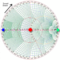
  • The red-dot in Fig. 2 corresponds to no reflection (50Ohm load, G=0) ; the blue-dot corresponds to short load (G=-1); the green-dot corresponds to open load (G=1).  The open load and short load is mirrored to each other through l/4 transformation as discussed in the next section.
Example:

Assume the characteristic impedance is 50Ω :

Z1 = 100 + j50Ω    Z2 = 75 - j100Ω    Z3 = j200Ω
Z4 = 150Ω  Z5 = ∞ (open)   Z6 = 0 (short)
Z7 = 50Ω   Z8 = 184 - j900Ω

smith chart3 

Fig. 3: Some Example Impedance

Note that a dipole antenna is close to open (Z5) at DC and becomes capacitive at lower frequency (Z8).  If it is well matched at operating frequency, the impedance is close to 50Ohm (Z7); that is: Z5->Z8->Z2->Z7.  Practically, the trajectory may be similar to the purple area because of non-perfect matching.


Transmission Line on Smith Chart

image 

Fig. 4: Input Impedance with Transmission Line

One key advantage of Smith Chart is to obtain the input impedance of a load with transmission line shown in the above figure. 

  • For a lossless transmission line, the input impedance toward source is simply a clockwise rotation of the load impedance on the Smith Chart shown in Fig. 2.  To remember clockwise rotation is to observe open load (green-dot) turns to capacitive (negative) load first; or short load (blue-dot) turns to inductive (positive) load first.
  • One full circle rotation on Smith Chart represents half-wavelength (l/2) transmission line length; half circle rotation represents l/4 line length.  Remember the famous quarter wavelength impedance transformation.  From open to short is half circle rotation, corresponds to l/4 transmission line length.  For any load after the l/4 transformation, the input impedance becomes the mirror point (with origin) on the Smith Chart.

Even though the Smith Chart is developed for system with transmission line, it is also very useful in lumped circuit for matching and analysis purpose in RF IC design  shown in next sections.


Admittance Smith Chart

The Smith chart is built by considering impedance (resistor and reactance).  Once the Smith chart is built, it can be used to analyze these parameters in both the series and parallel worlds.  Adding elements in a series is straightforward.  New elements can be added and their effects determined by simply moving along the circle to their respective values.  However, summing elements in parallel is another matter.  This requires considering additional parameters.  Often it is easier to work with parallel elements in the admittance world.

It turns out that the expression for y is the opposite, in sign, of z, and Γ(y) = -Γ(z).  If we know z, we can invert the signs of Γ and find a mirror point situated in the opposite direction.   Thus, an admittance Smith chart can be obtained by rotating the whole impedance Smith chart by 180°.  This is extremely convenient, as it eliminates the necessity of building another chart.  The intersecting point of all the circles (constant conductance and constant susceptances) is at the point (-1, 0) automatically.  With that plot, adding elements in parallel also becomes easier.  Math details can refer to this.


Lumped Elements on Smith Chart

When solving problems where elements in series and in parallel are mixed together, we can use the same Smith chart and rotate it around any point where conversions from z to y or y to z exist. 

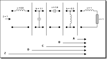
Let's consider the network of Fig. 5 (the elements are normalized with Z0 = 50Ω).  The series reactance (x) is positive for inductance and negative for capacitance. The susceptance (b) is positive for capacitance and negative for inductance.

image 

Fig. 5: Input Impedance of Lumped Elements

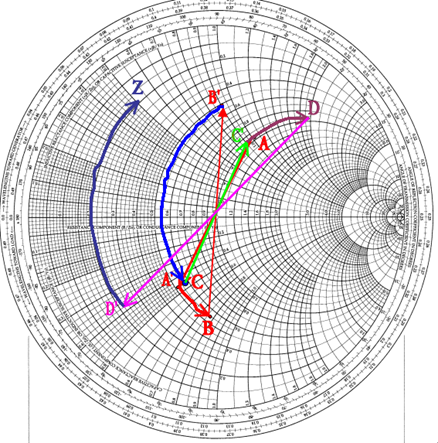
The circuit needs to be simplified (see Fig. 6).  Starting at the right side, where there is a resistor and an inductor with a value of 1, we plot a series point where the r circle = 1 and the l circle = 1.  This becomes point A.  As the next element is an element in shunt (parallel), we switch to the admittance Smith chart (by rotating the whole plane 180°).  To do this, however, we need to convert the previous point into admittance.  This becomes A'.  We then rotate the plane by 180°.  We are now in the admittance mode.  The shunt element can be added by going along the conductance circle by a distance corresponding to 0.3.  This must be done in a counterclockwise direction (negative value) and gives point B.  Fig. 7 shows the complete impedance transformation using Smith Chart.
image

Fig. 6: Break the Network for Analysis
image

Fig. 7: Impedance Using Smith Chart


In summary

1. Add a serial L:

Move up (clockwise) along  r=constant circle (circles intersects at (1,0))

2. Add a shunt L:

Move up (counter-clock) along g=constant circle (circles intersects at (-1,0))

3. Add a serial C:

Move down (counterclockwise) along r=constant circle (circles intersects at (1,0))

4. Add a shunt C:

Move  down (clockwise) along g=constant circle (circles intersects at (-1,0))

The following figure shows the summary.

image 


How to do matching using Smith Chart

L-match (8 types)

The following figure shows 4 different type of L match for positive reactance matching


image


Similarly, there are 4 types for negative reactance just exchange L and C.

pi/T-match

image


There are above 8 types of pi/T matching.  Similarly, the mirror from positive to negative is to change L and C.


Examples

(I) Impedance Transformation from Tom Lee's RF CMOS book.

* If ZL is a pure resistance and ZL > Zo; only type2 (shunt-C with serial-L, or shunt-L with serial C) can convert Zin < ZL and Zin = ZL / ??  (only at resonant frequency, normally is a LPF or  HPF)

* If ZL is a pure resistance and ZL < Zo; only type 4 (serial-C with shunt-L, or  serial C with shunt C) can convert Zin > ZL and Zin = ?? (only at resonant frequency, normally is a HPF)

The above two L matches are in Tom Lee's book.

(II)

For dipole antenna below resonating frequency, it is like a serial RLC resonator; the resistor is higher than 50Ohm (air is 270Ohm); typical may be  75Ohm.  The resonating  frequency is assumed to be higher than the desired frequency.   (Example, the LC frequency maybe 1GHz, but the operating frequency is 600MHz, etc.) 

Therefore, the impedance is  75+X j Ohm (X is -200 to -50 Ohm).  Is it possible to design a matching network? 

Before/after resonating frequency

Condition 1: Re > 50Ohm and Im < 0 (capacitive load with high real impedance): example: dipole antenna before resonator

Condition 2: Re < 50Ohm and Im > 0 (inductive load and low real impedance): example: loop antenna

Condition 3: Re > 50Ohm and Im > 0 (inductive load with high real impedance??): example: dipole antenna after the resonator?

Condition 4: Re < 50Ohm and Im < 0 (capacitive load with low real impedance??): example: loop antenna

The matching choice (a) serial inductor; (b) parallel inductor.  Both reduce the reactive part.  The problem of (a) is real part is not change.  Therefore choose (b) to reduce R from 72 to 50.  Then use a serial capacitor to bring to the right matching point!!!

The best way to do is to use the center frequency first, not considering the entire frequency range.  E.g. 400M to 800M, maybe use 600M for the matching purpose!!

Examine the L and Pi match

Impedance Matching with Smart Chart

http://www.maxim-ic.com/appnotes.cfm/an_pk/742/

  • Match for maximum power transfer or optimize the noise figure or highest gain?  Highest gain is always lowest noise figure?
  • Maximum power transfer => Rs = RL*
  • ?Ensure quality factor impact or access stability analysis because the matching network can be LPF or HPF or BPF.
  • ? Can we replace RLC with scattering wave analysis using smith chart for both passive and active component (cmos?)  there is no concept of impedance at low frequency? wrong, can I still normalize to 50Ohm since there is still finite value of impedance?

2011年2月13日 星期日

Matlab 替代方案

Matlab 毫無疑問是最常用的 computation 及 DSP 的軟體。大概也是我從大學以來使用程度最高的 programming language.  (其次是 perl,甚少用 C 或其它語言)  主要的好處 :

* Easy to use:  No malloc of array; matrix and vector operation; dynamic typing

* Complete DSP functions: windowing, fft, etc.

* Very nice graphics

主要的缺陷 :

1. Cost

2. Lack of general purpose programming language capability

3. Hard to integrate with other tools (such as verilog PLI) and do batch job.  Always need to open the matlab

I was looking for the right solution.   Octave is almost the same as Matlab as far as my work is concerned.  It only solved the cost part.

Pylab

Python is another alternative.   However, I found it’s difficult to use at beginning even with NumPy, SciPy, and Matplotlib.   For example, you need to do a=Vector([1, 2, 3]) instead of  a=[1,2,3].  Not mentioned to install the right tools.

The key is to Pylab (similar to Matlab) combines NumPy, SciPy, Matplotlib into an integrated  and consistent environment.  Pylab is an interactive mode of IPython (#ipython –pylab) similar to Matlab.

The most import thing is:

from pylab import *

Based on KeirMierle’s viewpoint, Pylab still needs to resolve these API consistency and installation issues.

Three Distributions Targeting Scientific Computing

Then I found the following three distributions based on Python

1. Sage: good for linux, maybe not easy for windows (use ?? as console)

2. Pythonxy: good for windows, maybe not good for linux (use Eclipse/IPython/Spyderlib as console)

3. Enthought Python Distribution (EPD): both for linux and windows.  The founder is the developer of NumPy (use IPython as console)

I found it’s very easy to use:

Cons:

1. First, the size of each distributin is huge.  For example, EPD 7.0 has 250MB.  Sage is similar, if not larger. 

2. EPD only support the lastest built.  EPD7.0 needs to use > glibc2.5.  That is, RHEL 5 or above.  For RHEL 4 you need to pay to get the old distribution.  Similar things may happen in other distribution.


Theerefore, alternative is to build your own environment (as many people have done it before).

The most essential part is: python, numpy, scipy, matplotlib, ipython (pylab), and maybe wxpython.


Installatin Procedure

Step1: Install python 2.6.5 (Matlibplot requires python 2.4-2.7) 

* Make sure installed python NOT overwrite /usr/bin/python since RHEL uses old python for lots of system scripts.

Step2: Use python2.6.5 to install easy_install for other python packages installation.

Step3: Use easy_install for NumPy

Step3b: Use easy_install for SciPy.  However, it seems to require fortran; encounter problems and skip.

Step4: Use easy_install for Matplotlib

* Matplotlib requires python 2.4-2.7

* NumPy 1.1 or later

* libpng 1.1 or later –> Use: “yum install libpng-devel”

* freetype 1.4 or later

Step5: Use easy_install for ipython

Step6: Add path (../bin before /usr/bin for python)

Run “ipython –pylab” for ipython in pylab mode.


The whole thing is summarized in the following shell script.

--------------------------------------------------------------------

#! /bin/sh

builddir=$(pwd)/pythondist
mkdir -p $builddir/source
cd $builddir/source

# Step1
wget 'http://python.org/ftp/python/2.6.5/Python-2.6.5.tgz'
wget 'http://pypi.python.org/packages/source/s/setuptools/setuptools-0.6c11.tar.gz#md5=7df2a529a074f613b509fb44feefe74e'
tar -xvzf Python-2.6.5.tgz

# Build python
cd $builddir/source/Python-2.6.5/

# The --prefix argument is the key!
./configure --prefix=$builddir

# Be sure to speed things up with the -j option if you're
# on a multicore machine (e.g. make -j 4 build for a quadcore)
make build
make install

# Step2
# Now install setuptools
cd $builddir/source
tar -xvzf setuptools-0.6c11.tar.gz
cd setuptools-0.6c11/

# The next key is to call this with the python you just built!
$builddir/bin/python setup.py build
$builddir/bin/python setup.py install

# Step3-5
# Now just install numpy, scipy, ipython, matplotlib, etc through easy_install
$builddir/bin/easy_install numpy
$builddir/bin/easy_install scipy
$builddir/bin/easy_install matplotlib
$builddir/bin/easy_install ipython

---------------------------------------------------------------------------------------------------


Testing Example

from pylab import *

x = linspace(0, 1000, 1024)

y = sin(x)

win = kaiser(x.size, 12)

plot(x, 20*log10(abs(fft(y*win))))

grid(1)

axis([0, 1, 0, 1])


Almost identical to matlab and very easy to use.

追蹤者